Practices

Databricks on AWS – An Architectural Perspective (part 1)

marzo 5, 2024 by Bluetab

Databricks on AWS – An Architectural Perspective (part 1)

Databricks has become a reference product in the field of unified analytics platforms for creating, deploying, sharing, and maintaining data solutions, providing an environment for engineering and analytical roles. Since not all organizations have the same types of workloads, Databricks has designed different plans that allow adaptation to various needs, and this has a direct impact on the architecture design of the platform.

With this series of articles, the goal is to address the integration of Databricks in AWS environments, analyzing the alternatives offered by the product in terms of architecture design. Additionally, the advantages of the Databricks platform itself will be discussed. Due to the extensive content, it has been considered convenient to divide them into three parts:

First installment:

Introduction.
Data Lakehouse & Delta.
Concepts.
Architecture.
Plans and types of workloads.
Networking.

Second installment:

Security.
Persistence.
Billing.

Introduction

Databricks is created with the idea of developing a unified environment where different profiles, such as Data Engineers, Data Scientists, and Data Analysts, can collaboratively work without the need for external service providers to offer the various functionalities each one needs in their daily tasks.

Databricks’ workspace provides a unified interface and tools for a variety of data tasks, including:

Programming and administration of data processing.
Dashboard generation and visualizations.
Management of security, governance, high availability, and disaster recovery.
Data exploration, annotation, and discovery.
Modeling, monitoring, and serving of Machine Learning (ML) models.
Generative AI solutions.

The birth of Databricks is made possible through the collaboration of the founders of Spark, who released Delta Lake and MLFlow as Databricks products following the open-source philosophy.

This new collaborative environment had a significant impact upon its introduction due to the innovations it offered by integrating different technologies:

Spark: A distributed programming framework known for its ability to perform queries on Delta Lakes at cost/time ratios superior to competitors, optimizing the analysis processes.
Delta Lake: Positioned as Spark’s storage support, Delta Lake combines the main advantages of Data Warehouses and Data Lakes by enabling the loading of both structured and unstructured information. It uses an enhanced version of Parquet that supports ACID transactions, ensuring the integrity of information in ETL processes carried out by Spark.
MLFlow: A platform for managing the end-to-end lifecycle of Machine Learning, including experimentation, reusability, centralized model deployment, and logging.

Data Lakehouse & Delta

A Data Lakehouse is a data management system that combines the benefits of Data Lakes and Data Warehouses.

A Data Lakehouse provides scalable storage and processing capabilities for modern organizations aiming to avoid isolated systems for processing different workloads such as Machine Learning (ML) and Business Intelligence (BI). A Data Lakehouse can help establish a single source of truth, eliminate redundant costs, and ensure data freshness.

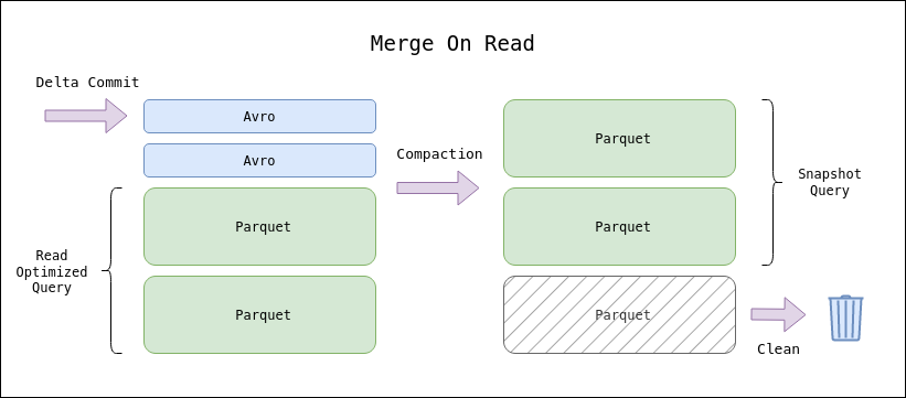
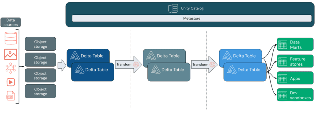
Data Lakehouses employ a data design pattern that gradually enhances and refines data as it moves through different layers. This pattern is often referred to as a medallion architecture.

Databricks relies on Apache Spark, a highly scalable engine that runs on compute resources decoupled from storage.

Databricks’ Data Lakehouse utilizes two key additional technologies:

Delta Lake: An optimized storage layer that supports ACID transactions and schema enforcement.
Unity Catalog: A unified and detailed governance solution for data and artificial intelligence.

Data Design Pattern:

Data Ingestion: In the ingestion layer, data arrives from various sources in batches or streams, in a wide range of formats. This initial stage provides an entry point for raw data. By converting these files into Delta tables, Delta Lake’s schema enforcement capabilities can be leveraged to identify and handle missing or unexpected data. Unity Catalog can be used to efficiently manage and log these tables based on data governance requirements and necessary security levels, allowing tracking of data lineage as it transforms and refines.

Processing, Cleaning, and Data Integration: After data verification, selection, and refinement take place. In this stage, data scientists and machine learning professionals often work with the data to combine, create new features, and complete cleaning. Once the data is fully cleaned, it can be integrated and reorganized into tables designed to meet specific business needs. The write-schema approach, along with Delta’s schema evolution capabilities, allows changes in this layer without rewriting the underlying logic providing data to end users.

Data Serving: The final layer provides clean and enriched data to end users. The end tables should be designed to meet all usage needs. Thanks to a unified governance model, data lineage can be tracked back to its single source of truth. Optimized data designs for various tasks enable users to access data for machine learning applications, data engineering, business intelligence, and reporting.

Features:

The Data Lakehouse concept leverages a Data Lake to store a wide variety of data in low-cost storage systems, such as Amazon S3 in this case.
Catalogs and schemas are used to provide governance and auditing mechanisms, allowing Data Manipulation Language (DML) operations through various languages, and storing change histories and data snapshots. Role-based access controls are applied to ensure security.
Performance and scalability optimization techniques are employed to ensure efficient system operation.
It allows the use of unstructured and non-SQL data, facilitating information exchange between platforms using open-source formats like Parquet and ORC, and offering APIs for efficient data access.
Provides end-to-end streaming support, eliminating the need for dedicated systems for real-time applications. This is complemented by parallel massive processing capabilities to handle diverse workloads and analyses efficiently.

Concepts: Account & Workspaces

In Databricks, a workspace is an implementation of Databricks in the cloud that serves as an environment for your team to access Databricks assets. You can choose to have multiple workspaces or just one, depending on your needs.

A Databricks account represents a single entity that can include multiple workspaces. Unity Catalog-enabled accounts can be used to centrally manage users and their data access across all workspaces in the account. Billing and support are also handled at the account level.

Billing: Databricks Units (DBUs)

Databricks invoices are based on Databricks Units (DBUs), processing capacity units per hour based on the type of VM instance.

Authentication & Authorization

Concepts related to Databricks identity management and access to Databricks assets.

User: A unique individual with access to the system. User identities are represented by email addresses.
Service Principal: Service identity for use with jobs, automated tools, and systems like scripts, applications, and CI/CD platforms. Service entities are represented by an application ID.
Group: A collection of identities. Groups simplify identity management, making it easier to assign access to workspaces, data, and other objects. All Databricks identities can be assigned as group members.
Access control list (ACL): A list of permissions associated with the workspace, cluster, job, table, or experiment. An ACL specifies which users or system processes are granted access to objects and what operations are allowed on the assets. Each entry in a typical ACL specifies a principal and an operation.
Personal access token: A opaque string for authenticating with the REST API, SQL warehouses, etc.
UI (User Interface): Databricks user interface, a graphical interface for interacting with features such as workspace folders and their contained objects, data objects, and computational resources.

Data Science & Engineering

Tools for data engineering and data science collaboration.

Workspace: An environment to access all Databricks assets, organizing objects (Notebooks, libraries, dashboards, and experiments) into folders and providing access to data objects and computational resources.
Notebook: A web-based interface for creating data science and machine learning workflows containing executable commands, visualizations, and narrative text.
Dashboard: An interface providing organized access to visualizations.
Library: A available code package that runs on the cluster. Databricks includes many libraries, and custom ones can be added.
Repo: A folder whose contents are versioned together by synchronizing them with a remote Git repository. Databricks Repos integrates with Git to provide source code control and versioning for projects.
Experiment: A collection of MLflow runs to train a machine learning model.

Databricks Interfaces

Describes the interfaces Databricks supports in addition to the user interface to access its assets: API and Command Line Interface (CLI).

REST API: Databricks provides API documentation for the workspace and account.
CLI: Open-source project hosted on GitHub. The CLI is based on Databricks REST API.

Data Management

Describes objects containing the data on which analysis is performed and feeds machine learning algorithms.

Databricks File System (DBFS): Abstraction layer over a blob store. It contains directories, which can hold files (data files, libraries, and images) and other directories.
Database: A collection of data objects such as tables or views and functions, organized for easy access, management, and updating.
Table: Representation of structured data.
Delta table: By default, all tables created in Databricks are Delta tables. Delta tables are based on the open-source Delta Lake project, a framework for high-performance ACID table storage in cloud object stores.
Metastore: Component storing all the structure information of different tables and partitions in the data store, including column and column type information, serializers and deserializers needed to read and write data, and the corresponding files where data is stored.
Visualization: Graphical representation of the result of executing a query.

Computation Management

Describes concepts for executing computations in Databricks.

Cluster: A set of configurations and computing resources where Notebooks and jobs run. There are two types of clusters: all-purpose and job.
- An all-purpose cluster is created manually through the UI, CLI, or REST API and can be manually terminated and restarted.
- A job cluster is created when running a job on a new job cluster and terminates when the job is completed. Job clusters cannot be restarted.
Pool: A set of instances ready for use that reduces cluster start times and enables automatic scaling. When attached to a pool, a cluster assigns driver and worker nodes to the pool. If the pool doesn’t have enough resources to handle the cluster’s request, the pool expands by assigning new instances from the instance provider.
Databricks Runtime: A set of core components running on clusters managed by Databricks. There are several runtimes available:
- Databricks runtime includes Apache Spark and adds components and updates to improve usability, performance, and security.
- Databricks runtime for Machine Learning is based on Databricks runtime and provides a pre-built machine learning infrastructure that integrates with all Databricks workspace capabilities.

Workflows

Frameworks for developing and running data processing pipelines:

Jobs: Non-interactive mechanism to run a Notebook or library either immediately or on a schedule.
Delta Live Tables: Framework for creating reliable, maintainable, and auditable data processing pipelines.
Workload: Databricks identifies two types of workloads subject to different pricing schemes:
- Data Engineering (job): An (automated) workload running on a job cluster that Databricks creates for each workload.
- Data Analysis (all-purpose): An (interactive) workload running on an all-purpose cluster. Interactive workloads typically execute commands within Databricks Notebooks.
Execution context: State of a Read-Eval-Print Loop (REPL) environment for each supported programming language. Supported languages are Python, R, Scala, and SQL.

Machine Learning

End-to-end integrated environment incorporating managed services for experiment tracking, model training, function development and management, and serving functions and models.

Experiments: Primary unit of organization for tracking the development of machine learning models.
Feature Store: Centralized repository of features enabling sharing and discovery of functions across the organization, ensuring the same function calculation code is used for both model training and inference.
Models & model registry: Machine learning or deep learning model registered in the model registry.

SQL

SQL REST API: Interface allowing automation of tasks on SQL objects.
Dashboard: Representation of data visualizations and comments.
SQL queries: SQL queries in Databricks.
- Query: SQL query.
- SQL warehouse: SQL storage.
- Query history: History of queries.

Architecture: High-level architecture

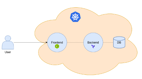
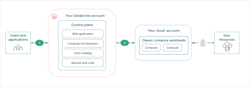
Before we start analyzing the various alternatives that Databricks offers for infrastructure deployment, it is advisable to understand the main components of the product. Below is a high-level overview of the Databricks architecture, including its enterprise architecture, in conjunction with AWS.

Although architectures may vary based on custom configurations, the above diagram represents the structure and most common data flow for Databricks in AWS environments.

The diagram outlines the general architecture of the classic compute plane. Regarding the architecture for the serverless compute plane used for serverless SQL pools, the compute layer is hosted in a Databricks account instead of an AWS account.

Control plane and compute plane:

Databricks is structured to enable secure collaboration in multifunctional teams while maintaining a significant number of backend services managed by Databricks. This allows you to focus on data science, data analysis, and data engineering tasks.

The control plane includes backend services that Databricks manages in its Databricks account. Notebooks and many other workspace configurations are stored in the control plane and encrypted at rest.
The compute plane is where data is processed.

For most Databricks computations, computing resources are in your AWS account, referred to as the classic compute plane. This pertains to the network in your AWS account and its resources. Databricks uses the classic compute plane for its Notebooks, jobs, and classic and professional Databricks SQL pools.

As mentioned earlier, for serverless SQL pools, serverless computing resources run in a serverless compute plane in a Databricks account.

Databricks has numerous connectors to link clusters to external data sources outside the AWS account for data ingestion or storage. These connectors also facilitate ingesting data from external streaming sources such as event data, streaming data, IoT data, etc.

The Data Lake is stored at rest in the AWS account and in the data sources themselves to maintain control and ownership of the data.

E2 Architecture:

The E2 platform provides features like:

Multi-workspace accounts.
Customer-managed VPCs: Creating Databricks workspaces in your VPC instead of using the default architecture where clusters are created in a single AWS VPC that Databricks creates and configures in your AWS account.
Secure cluster connectivity: Also known as “No Public IPs,” secure cluster connectivity allows launching clusters where all nodes have private IP addresses, providing enhanced security.
Customer-managed keys: Provide KMS keys for data encryption.

Workload plans and types

The price indicated by Databricks is attributed in relation to the DBUs consumed by the clusters. This parameter is associated with the processing capacity consumed by the clusters and directly depends on the type of instances selected (when configuring the cluster, an approximate calculation of the DBUs it will consume per hour is provided).

The price charged per DBU depends on two main factors:

Computational factor: the definition of cluster characteristics (Cluster Mode, Runtime, On-Demand-Spot Instances, Autoscaling, etc.) that will result in the allocation of a specific package.
Architecture factor: customization of this (Customer Managed-VPC), in some aspects may require a Premium or even Enterprise subscription, causing the cost of each DBU to be higher as you obtain a subscription with greater privileges.

The combination of both computational and architectural factors will determine the final cost of each DBU per hour of operation.

All information regarding plans and types of work can be found at the following link

Networking

Databricks has an architecture divided into control plane and compute plane. The control plane includes backend services managed by Databricks, while the compute plane processes the data. For classic computing and calculation, resources are in the AWS account in a classic compute plane. For serverless computing, resources run on a serverless compute plane in the Databricks account.

Thus, Databricks provides secure network connectivity by default, but additional features can be configured. Key points include:

Connection between users and Databricks: This can be controlled and configured for private connectivity. Configurable features include:
- Authentication and access control.
- Private connection.
- Access IP list.
- Firewall rules.
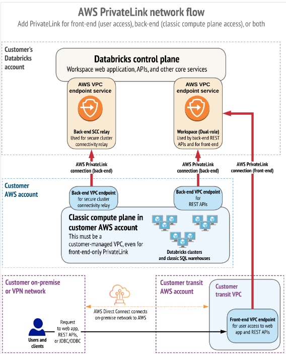
Network connectivity features for the control plane and compute plane. Connectivity between the control plane and the serverless compute plane is always done through the cloud network, not over the public Internet. This approach focuses on establishing and securing the connection between the control plane and the classic compute plane. The concept of ‘secure cluster connectivity’ is worth noting, where, when enabled, the client’s virtual networks have no open ports, and Databricks cluster nodes do not have public IP addresses, simplifying network management. Additionally, there is the option to deploy a workspace within the Virtual Private Cloud (VPC) on AWS, providing greater control over the AWS account and limiting outbound connections. Other topics include the possibility of pairing the Databricks VPC with another AWS VPC for added security, and enabling private connectivity from the control plane to the classic compute plane through AWS PrivateLink.”

The following link is provided for more information on these specific features.

Connections through Private Network (Private Links)

Finally, we want to highlight how AWS uses PrivateLinks to establish private connectivity between users and Databricks workspaces, as well as between clusters and the infrastructure of the workspaces.

AWS PrivateLink provides private connectivity from AWS VPCs and on-premises networks to AWS services without exposing the traffic to the public network. In Databricks, PrivateLink connections are supported for two types of connections: Front-end (users to workspaces) and back-end (control plane to control plane).

The front-end connection allows users to connect to the web application, REST API, and Databricks Connect through a VPC interface endpoint.

The back-end connection means that Databricks Runtime clusters in a customer-managed VPC connect to the central services of the workspace in the Databricks account to access the REST APIs.

Both PrivateLink connections or only one of them can be implemented.

Referencias

What is a data lakehouse? [link] (January 18, 2024)

Databricks concepts [link] (January 31, 2024)

Architecture [link] (December 18, 2023)

Users to Databricks networking [link] (February 7, 2024)

Secure cluster connectivity [link] (January 23, 2024)

Enable AWS PrivateLink [link] (February 06, 2024)

Do you want to know more about what we offer and to see other success stories?

SOLUTIONS, WE ARE EXPERTS

DATA STRATEGY

DATA FABRIC

AUGMENTED ANALYTICS

Mi experiencia en el mundo de Big Data – Parte II

febrero 4, 2022

Gobierno de Datos: ¿tendencia o necesidad?

octubre 13, 2022

Guía avanzada sobre almacenamiento en Snowflake

octubre 3, 2022

Bluetab en la ElixirConfEU 2023

mayo 3, 2023

Hashicorp Boundary

diciembre 3, 2020

Análisis de vulnerabilidades en contenedores con trivy

marzo 22, 2024

LakeHouse Streaming on AWS with Apache Flink and Hudi (Part 2)

octubre 4, 2023 by Bluetab

LakeHouse Streaming on AWS with Apache Flink and Hudi (Part 2)

Introduction

This article is the second in a series of publications focusing on the creation of a LakeHouse with Hudi from a streaming ingest processed by a Flink application. The first article focuses on laying a good foundation for this platform, where Flink applications were deployed with KDA (Kinesis Data Analytics) for each type of format (MoR, CoW for Hudi and JSON) that write the result of this processing into buckets.

The input data was sent in the previous article from a local machine running a Locust application, which can present problems when scaling and processing a high volume of events. In addition, Kinesis Data Analytics applications with Flink present agility problems in their auto-scaling mode. All these new challenges will be solved in this article.

These tables will also be cataloged in Glue, a service that provides a data catalog in AWS, in order to access them and perform queries of all kinds. The query engine that will consume this metadata will be Athena, which provides a scalable, agile and serverless experience to be able to execute queries with SQL or Spark for our tables hosted in S3.

On the other hand, in this article we have also deployed the necessary components to be able to monitor our applications and thus draw conclusions about the speed at which data is ingested and the possible problems to be solved so that the processing has the required latency according to the requirements imposed.

Finally, a performance and latency comparison of the different Flink applications that write data in Hudi and JSON formats will be made in order to see the different advantages and disadvantages of these formats.

Architecture

Below you can see the high-level architecture that will be deployed:

For a better understanding we are going to explain it from left to right. As you can see, the most notable change with respect to the first article is the inclusion of a Kubernetes cluster to be able to scale the events that will be sent as input to our streaming application. In this way, it will be possible to thoroughly test the performance of Flink applications depending on their provisioning and especially on the type of format and table in which they write to the LakeHouse. In addition, an ALB (Application Load Balancer) has been made available to access the Locust interface to define the number of users to simulate and how they should scale over time. The URL to access this will appear as output when deploying the infrastructure with Terraform.

On the other hand, significant changes have been made to the Flink KDA applications and the stream they read from. Each application now reads as EFO (Enhanced Fan Out) consumers, so that each of them has a dedicated bandwidth. The reason for this change and its details will be explained in more detail in the dedicated section for Kinesis.

Regarding the monitoring and extraction of metrics in NRT (Near Real Time), lambdas functions have been deployed that query the tables based on Athena thanks to having registered the metadata of these tables in the Glue catalog. It is important to note that the metadata of Hudi tables are registered in Glue by Flink but in the case of JSON a crawler is deployed that registers these tables in the catalog. This crawler must be executed manually for this table to be registered in Glue.

Scaling

Kinesis Stream

Since the goal is to subject the application to a considerable load of events per second, it is necessary to explain how each of the pieces of the architecture can scale according to the volume of data.

As previously mentioned, a Kinesis Stream On-Demand has been chosen to automate the scaling of the shards during load testing. It should be noted that these streams can accommodate a write rate of up to 200% of that specified by the number of shards at any given time.

Once the stream is above 100%, it will automatically increase the number of shards within 15 minutes. The only limitation is therefore not to exceed twice the supported write volume in less than that period.

On the other hand, since you will have three Flink applications reading from the same stream, read limitations will be the biggest problem. A Kinesis Stream only supports 5 GetRecord calls per shard per second. Since each application has to read the entire stream (and therefore all shards), increasing the number of shards does not help to solve this problem.

The solution is to register each application as an Enhanced Fan-Out consumer. This functionality of the Kinesis Stream provides each of these consumers with an individual limit of 5 GetRecord calls and 2MB per shard per second of reading.

This configuration is done on the consumer side, in our case via the Kinesis connector for Flink:

'scan.stream.recordpublisher' = 'EFO',
'scan.stream.efo.registration' = 'EAGER/LAZY',
'scan.stream.efo.consumername' = '{consumer_name}'

It is worth mentioning that alternatively, it is possible to increase the read latency of our Flink applications. By default Flink performs a read every 200ms per shard, so one application completely consumes the read quota of a stream. By increasing this value to 600ms we could accommodate all three applications, at the cost of increased latency:

scan.shard.getrecords.intervalmillis = '600'

Use will also be made of the Adaptive Reads option, which dynamically modifies the number of events collected per call depending on the size of each record. This makes it possible to take advantage of the 2 MB/s per shard available for each consumer:

'scan.shard.adaptivereads' = 'true'

Regarding scaling in Flink KPUs (Kinesis Processing Unit), we have chosen not to make use of autoscaling, since each scaling process incurs in downtime for the application. Due to the different requirements of each of the applications, scaling actions at unexpected times could interrupt load testing. In addition, it is interesting to measure the write performance of each of the applications at equal computing capacity.

Hudi

Timeline

One of the basic systems on which Hudi’s operation and features are based is the timeline. Hudi keeps a temporary record of all the actions that have been performed on the table, as well as the status of this action.

The main actions that make up the timeline are as follows

Commits – atomic writing of a set of records to the table in columnar format
Delta Commit – similar to commit, represents a write of records in the form of logs to a Merge on Read table.
Compaction – compaction of log writes (delta commits) from a MoR table to columnar format
Cleans – deletion of old versions of files
Rollback – deleted from records written by a failed commit or delta commit
Savepoint – marks a set of files as «saved» so that they will not be deleted by the cleanup process. Allows to restore the table to a previous point in the timeline.

Any of these actions can be found in one of three states

Requested – an action has been planned but not yet started
Inflight – the action is in progress
Completed – denotes that the action has been completed.

Table types

As hinted in the operation of the Hudi timeline, there are two types of writing supported: columnar and logs. The columnar (parquet) format constitutes the final form of a Hudi table, together with the timeline metadata. However, it is possible to make use of log writes (avro) to decrease the write latency and eventually compact to columnar format without hindering the write.

The use of these writing methods gives rise to the two types of table that Hudi makes available to us

Copy on Write – writes are performed exclusively in columnar format, creating a new file with the new table records. The data is available immediately but incurs higher write latency.
Merge on Read – makes use of writing to logs. The new records are initially written as logs, and will later be transformed to columnar format by the compaction process. We obtain lower write latency at the cost of read latency; the new logs will not be available until compaction is performed.

Query Types

In order to take advantage of the characteristics of each type of table, there are three types of queries that can be performed on a Hudi table

Snapshot – obtains the latest version of the table. For MoR tables this involves incurring a compaction process to get the latest records in log format.
Read Optimized – for MoR tables, reads only the records already exposed in columnar format without incurring additional read latency.
Incremental – collects only new records since a certain commit or compact, facilitating the creation of incremental pipelines. Not supported by Athena

Integration with Glue Catalog

The Hudi connector allows a native integration with the Glue catalog in AWS. Simply add the Hive dependencies in our Flink application:

com.amazonaws.aws-java-sdk-glue
org.apache.hive.hive-common
org.apache.hive.hive-exec

And specify the catalog configuration in the Hudi connector:

'hive_sync.enable' = 'true',
'hive_sync.db' = '{glue_database}',
'hive_sync.table' = '{table_name}',
'hive_sync.partition_fields' = '{partition_fields}',
'hive_sync.mode' = 'glue',
'hive_sync.use_jdbc' = 'false'

With this integration, the application will automatically create the tables in the catalog. As mentioned before, there are different types of queries to query a Hudi table. Therefore, different tables will be created in the catalog to support the different queries.

For a CoW table, the table will be queried using a Snapshot query. For MoR on the other hand, two tables will be made available to support Read Optimized or Snapshot queries.

The main application of Glue is to support lambdas so that when executing queries through Athena their execution can be done in a more efficient, fast and secure way:

Glue Catalog: centralized storage of information about the organization, design and format of the data, used by Athena to directly perform queries to S3 without having to rely on third parties to obtain this information.
Schema Automation: Glue automatically tracks and catalogs data in S3, detecting and adapting schema changes. This avoids possible errors and allows the reading of new fields in case of alterations in the event schemas.

Hudi configuration

It is important to understand the configurations offered by Hudi to optimize our application, in particular for a Near Real Time application it is convenient to be aware of the available options. Although the configuration capacity is immense [1], we will try to summarize the most relevant ones for a first contact with this technology.

Partitioning

Apache Hudi offers the types of partitioning that can be found in other solutions, the main ones will be detailed and the implemented one will be justified:

Simple: partitioning based on a single field, in this case the field chosen is ‘ticker’ as it has been identified as the one with the lowest cardinality.

Compound Partitioning: partitioning based on multiple fields, it could be interesting to choose a low cardinality field (ticker) and a medium cardinality field (date).

Dynamic Partitioning: choice of the variable based on the values, it can be interesting when the cardinality of the variables can undergo variations and an update of the partitioning is required in an automatic and flexible way.

Indexes

Apache Hudi has multiple types of indexing [2], we will briefly discuss the most common ones:

Bloom Index – Makes use of a bloom filter on the key of the events, additionally it can be complemented with a filtering by key range. It works well when dealing with a table where most changes occur in the most recent partitions or for event deduplication.
Simple: indexing performed by the combination of FileID and RecordKey. Recommended when Upsert operations are not so frequent due to the simplicity it offers.

Both types of indexes can be used in their global form

Global index – They impose the uniqueness of the keys in all the partitions of the table, that is to say, they guarantee that there will be only one record with a certain key.
Non-global index – Key uniqueness is only required at the partition level. If the data is consistent and a key is only going to exist in one partition, this type of index offers much better performance and better scaling.

In this case, a Bloom Index has been chosen, which is the default in case it is not expressly stated:

"hoodie.index.type" = "BLOOM"

The choice of this type of indexing is due to the fact that the use cases that have been raised require a considerably high and efficient data processing.

Types of operations

Apache Hudi offers several types of operations [3] that allow users to manage and modify large data sets. The main operations performed in Stress Tests as well as in other scenarios are detailed below:

Upsert – This is the default operation, and will execute an insert or an update depending on whether the record already exists after an index lookup. With this operation the table will have no duplicates for its primary key.
Insert – This operation ignores the index lookup when inserting events. It is the fastest but the table may contain duplicates. It is still useful if auxiliary deduplication methods are used, or simply the existence of these is tolerable in the use case.
Delete: Hudi offers two deletion methods. Soft Delete converts to null the values of the event except for the key. Hard Delete executes a physical deletion of the event in the table.
Bulk Insert Operation similar to Insert but optimized for insertion of a large volume of data, at the cost of sacrificing some guarantees in file size control. Scales well for hundreds of TBs in case of initial bootstrap of a large table.

Compaction

In the case of using a MoR table, it is possible to configure the log compaction rate to find the balance between write and read latency that best suits the use case. It is possible to specify a strategy of time or number of delta commits (or both) that execute a compaction process:

compaction.delta_commits
compaction.delta_seconds
compaction.trigger.strategy

Asynchronous actions

Certain timeline actions such as compacting, cleaning, archiving and clustering can be performed asynchronously by the application, or even relegated to auxiliary processes to the writing application. In the case of Flink, it can help improve write latency and avoid BackPressure problems in the application:

compaction.async.enabled
hoodie.clean.async
hoodie.archive.async
hoodie.clustering.async.enabled

Stress Tests & Insights

When deploying the applications, different tests have been performed, varying both the maximum load of events and the concurrency and exponential degree of growth of the same. This has been possible thanks to the flexibility offered by Locust being built on a Kubernetes cluster, being able to set a maximum limit of concurrency of events and an incremental of them. In the tests, a maximum limit of 5 to 15K simultaneous users (Peak Concurrency) has been established, scaling the frequency of the same in a linear way, from 5 to 20 more users per second (Spawn Rate):

The different tests have been monitored in order to draw conclusions about the performance, taking into account the specific characteristics of each of the formats. The metrics on which the analyses have been based are both the native CloudWatch Metrics (CPU & Memory Utilization, KPUs, LastCheckpoint SIze & Duration,…), as well as the metrics obtained from the Lambdas that periodically consult the number of events available in the buckets and calculate the average latency of the same.

Number of Events

When analyzing the total number of events processed, which are sent gradually, i.e., as time passes more and more events are sent per second, a fairly similar trend is identified although JSON and Hudi MoR stand out over Hudi CoW in terms of performance. It is worth noting that JSON shows a more stable and steady growth compared to Hudi MoR and CoW and this is because the latter are able to handle incremental updates in the data.

The similarity between JSON and Hudi MoR makes the choice entirely based on the characteristics of the project. In case the data is not updated JSON may be a more interesting solution mainly due to its simplicity, while if there is a high frequency of historical data update, Hudi MoR may be a better solution. This is due both to the higher efficiency in reading tasks and because of the possibility to record different versions of the data.

Latency

Due to the difficulty of standardizing the latency calculation logic between 3 different types of storage, we have chosen to simplify it by calculating it as the difference between the time of event creation and the time of processing in the respective application.

Similar behavior is observed between JSON and Hudi MoR, although the former in a more critical way, having a very low initial latency but as both processing time and load volume increases, this latency is negatively affected.

The choice between JSON and Hudi MoR will depend both on the fault tolerance of the application and the characteristics of each of the formats, in case the data structure is stable and does not change frequently, or does not depend on incremental updates and can deal with complete rewrites, then JSON may be a better choice.

The choice of Hudi CoW over MoR can be made when high error tolerance and high recoverability from failed or corrupted write events are required.

CPU utilization

When analyzing CPU usage, a certain homogeneity has been identified among the different tests, even when working with different workloads. JSON and Hudi MoR stand out for having the lowest CPU usage levels, both for different reasons. JSON stands out for its simplicity by directly including the new data without having to deal with data versioning, while MoR does not consume as much CPU since, due to its characteristics, the highest CPU consumption is made when performing read queries, in the write tasks it only identifies the changes that will be applied when querying them.

Remember that CloudWatch native metrics only allow us to monitor the applications, which correspond to the writing tasks. The monitoring of read tasks corresponds to the Lambdas mentioned above.

In this case MoR is more beneficial with respect to CoW, since the higher CPU consumption in MoR occurs when querying the stored data while in CoW it occurs when updating the data.

The choice between the most efficient formats depends on the needs of the project, in case a higher fault tolerance, data versioning and higher reading efficiency are required, MoR will be chosen over JSON, between the two Hudi formats, again, the choice will depend on the characteristics of the project, if the queries require heavy and/or complex transformations, MoR would be chosen; if, on the other hand, the project requires greater data integrity and/or the data ingestion is in batch, CoW would be more interesting because when working with these volumes of data, having backup copies, in case of errors, the impact in terms of costs and recovery time is lower.

Memory Utilization

JSON again stands out for having the lowest memory usage values, although for the number of transformations that are performed, they are relatively high, especially considering that it does not have to deal with version management or data merging. These values are due to the fact that it does not have optimized compression capabilities or efficient schema management.

Regarding Hudi, similar conclusions can be drawn as in the CPU usage section, MoR has a higher memory utilization than JSON due to delta log processing and version management and a lower one to CoW since the actual data consolidation does not occur during writing.

Last Checkpoint Size

It is important to highlight, once again, the stability of JSON compared to Hudi applications, since it not only shows a lower value than both in the tests performed, but also a stability that is not achieved with either MoR or CoW, since, as can be seen, when monitoring the size of the Checkpoints, considerable volatility is perceived.

Perceived volatility in Hudi applications is mainly due to Checkpoint failures, which leads to a larger Checkpoint volume after the failure. In addition to this, the volatility in Checkpoint sizes may be related to the optimization and compaction operations performed internally that may lead to state compaction, which considerably reduces the size of the Checkpoint.

Development challenges

Read Throughput of Kinesis and EFO

In order not to exceed the read limit on the Kinesis Stream we have chosen to subscribe the consumers as Enhanced Fan-Out. In some tests in conjunction with Autoscaling this has given problems with the Flink Kinesis connector being unable to close connections when scaling the cluster.

Hudi configuration

Hudi’s configuration has been another sticking point during development. Under high loads the compaction and cleanup processes are more likely to cause backpressure problems and cause application errors. Although configuring these processes to occur asynchronously can alleviate this problem, conflicts and misalignment between processes can arise under high loads. A balance between these configurations and the application’s cluster capacity are key to the smooth operation of the application.

Format heterogeneity

When analyzing the performance of the 3 applications, there is an additional difficulty due to the nature of the format types, which has an impact both on the architecture and on the development of the logics.

The different behavior of the formats in the ingest complicates the development oflogics when calculating latency. MoR writes to logs after compaction, so the data is not immediately available as is the case with CoW or JSON. This implies that the common measurable metric for all formats is read availability, which is not the main purpose of a MoR table.

Synchronization with the Glue Catalog

One of the great advantages we have found with Hudi is its ability to synchronize with the Glue catalog, creating the tables and keeping them updated without the need for a crawler. This allows for a cleaner application and architecture than in the case of JSON, for which it must be run manually when deploying applications.

Conclusions

The test results show considerable differences between the JSON, Hudi MoR and CoW formats in terms of efficiency, responsiveness and resource utilization. We proceed to analyze each of the aspects in more detail:

Processing Efficiency: JSON and Hudi MoR stand out in most metrics, showing optimal performance in terms of Latency, CPU & Memory Utilization. However, JSON behavior is more stable and predictable, although MoR has advantages over JSON, for example, in incremental update management.
Resilience and Fault Tolerance: fault tolerance is a very important factor in the decision on the choice between Hudi and JSON. In the case of MoR and CoW, it will depend on the degree of criticality, since at a general level the performance in writing tasks for MoR is superior.
Resource Usage: JSON is shown to be the most lightweight, with low CPU and memory utilization, due to its inherent simplicity. Whereas Hudi MoR and CoW, due to the nature of their design and data management, require more resources, especially in operations involving version management and data compaction.

Finally, it is interesting to identify in which use cases or projects each of the formats may be more recommendable depending on their characteristics and the network flags that may be established:

JSON: Recommended for applications with stable data structures that do not require incremental updates and where simplicity and stability are key.
Hudi MoR: Suitable for projects that require efficient management of incremental updates and where latency and writing efficiency are crucial.
Hudi CoW: Ideal for contexts where data integrity is essential, and robust error recovery is needed, especially in batch ingest scenarios.

References

[1] Hudi Tables Configuration. [link]

[2] Index Types in Hudi. [link]

[3] Hudi Operation Types. [link]

Autores

I started my career with the development, maintenance and administration of multidimensional databases and Data Lakes. From there I started to be interested in data platforms and cloud architectures, being certified 3 times in AWS and 2 with Hashicorp.

I am currently working as a Cloud Engineer developing Data Lakes and DataWarehouses with AWS for a client related to the organization of sporting events worldwide.

Passionate about data and new technologies, specialized as AWS Cloud Engineer in DataWarehouses optimization and Data Lakes ingestion and transformation processes. Motivated by continuous improvement and automation of service integration.

Actively collaborating with the Cloud Practice group in research and blog development of cutting-edge and innovative technologies such as this one, thus fostering continuous learning.

Dedicated to constantly learning new technologies and their application, enjoying using them to solve technological challenges. I develop my career as a Cloud Engineer designing, implementing and maintaining infrastructure in AWS.

I actively collaborate in the Cloud Practice, where we research and experiment with new technologies, seeking solutions to the challenges faced by our clients.

¿Quieres saber más de lo que ofrecemos y ver otros casos de éxito?

SOLUCIONES, SOMOS EXPERTOS

DATA STRATEGY

DATA FABRIC

AUGMENTED ANALYTICS

Te puede interesar

Azure Data Studio y Copilot

octubre 11, 2023

Serverless Microservices

octubre 14, 2021

Espiando a tu kubernetes con kubewatch

septiembre 14, 2020

Data Mesh

julio 27, 2022

El futuro del Cloud y GenIA en el Next ’23

septiembre 19, 2023

Usando los Grandes Modelos de Lenguaje en información privada

marzo 11, 2024

Starburst: Construyendo un futuro basado en datos.

mayo 25, 2023 by Bluetab

Starburst: Construyendo un futuro basado en datos.

Introducción

En este nuevo artículo vamos a hablar de uno de nuestros partners: Starburst[1]. Starburst es la versión empresarial de Trino[2] realizando nuevas integraciones, mejoras de rendimiento, una capa de seguridad y restando complejidad a la gestión con una interfaz de usuario muy fácil de usar y que te permite realizar distintas configuraciones.

Para los que no conocéis Trino, es un motor de consulta SQL distribuido open-source creado en 2012 por Facebook bajo el nombre Presto. Está diseñado para consultar grandes conjuntos de datos distribuidos en una o más fuentes de datos heterogéneas. Esto significa que podemos consultar datos que residen en diferentes sistemas de almacenamiento como HDFS, AWS S3, Google Cloud Storage o Azure Blob Storage. Trino también tiene la capacidad de federar diferentes fuentes de datos como MySQL, PostgreSQL, Cassandra, Kafka.

Con las nuevas necesidades que van saliendo de arquitecturas orientadas al Data Mesh[3], plataformas analíticas como Starburst son cada vez más importantes y nos permiten centralizar y federar distintas fuentes de datos para así tener solo un punto de entrada a nuestra información. Con esta mentalidad, podemos hacer que nuestros usuarios accedan a la plataforma de Starburst con distintos roles y distinta granularidad de acceso para que puedan consultar los distintos dominios que poseen las empresas. Además Starburst no solo se queda en la consulta de datos, sino que nos permite conectarnos con herramientas analíticas como puedes ser DBT[4] o Jupyter Notebook[5] o herramientas de reporting como Power BI[6] para sacarle más rendimiento a todos nuestros datos. Pero Starburst no solo se queda en eso, sino que nos puede ayudar en la migraciones de datos hacia el Cloud, ya que fácilmente podemos conectarnos a las fuentes de datos y sacar toda la información para volcarlas en cualquier almacenamiento del Cloud.

Como podéis observar, Starburst es capaz de analizar todos sus datos, dentro y alrededor de tu Data Lake, y se conecta a todo un ecosistema de herramientas. Por eso vamos a realizar una serie de artículos para tratar los puntos más relevantes como son el despliegue y configuración de la plataforma, integración con otras herramientas y gobierno y administración de usuarios. En este primer artículo, nos vamos a centrar en el despliegue de Starburst en Kubernetes, así como la configuración que se tiene que realizar para conectar con los distintos componentes de GCP. Además hemos añadido una capa de monitorización con Prometheus[7] y Grafana[8], donde hemos publicado un dashboard con distintas métricas importantes por si cualquier compañía quiere centralizar las métricas en Grafana. Para todo ello, nos vamos a apoyar de un repositorio que hemos creado con el levantamiento de la infraestructura y la instalación de Starburst.

¿Qué necesitas para entender este artículo?

Algunos conceptos sobre Terraform[9].
Algunos conceptos de Kubernetes.
Algunos conceptos de Helm.
Algunos conceptos de Prometheus.
Algunos conceptos de Grafana.
Un cuenta en GCP.
Una licencia de Starburst

Arquitectura

Como se puede observar en el diagrama, estos son los componentes que se van a desplegar para la configuración de Starburst. Como pieza central del despliegue, utilizaremos Google Kubernetes Engine. Este es el servicio administrado de orquestación de contenedores de Google. Utilizaremos Kubernetes ya que nos facilitará la gestión de Starburst y aprovecharemos las ventajas del autoscaling de Kubernetes para ampliar el número de workers de Starburst y escalar en más nodos para poder así tener más recursos de computación si tenemos algún pico de trabajo o de usuarios.

Como configuración inicial de nuestro cluster de GKE, comenzaremos con un único nodepool para facilitar el despliegue. Un nodepool es una agrupación de nodos dentro de un cluster con la misma configuración y especificaciones de tipo de máquina. En nuestro caso, nuestro nodepool se llamará `default-node-pool` y el tipo de instancia utilizada será `e2-standard-16`, que es la recomendada por Starburst, ya que el tipo de carga de trabajo necesita nodos con bastante memoria. Además de la instalación de Starburst, también desplegaremos en el cluster tanto Prometheus como Grafana.

Como hemos explicado anteriormente, Starburst está basado en Trino, que es un motor de consulta distribuido. Los principales componentes de Trino son el Coordinator y los Workers. El Coordinator de Trino es el componente responsable de analizar las sentencias, planificar las consultas y gestionar los nodos Workers de Trino. El Coordinator realiza un seguimiento de la actividad de cada Worker y orquesta la ejecución de una consulta. Los Workers son el componente responsable de ejecutar tareas y procesar datos. Los nodos Workers obtienen datos de los conectores e intercambian datos intermedios entre sí. El Coordinator es responsable de obtener los resultados de los Workers y devolver los resultados finales al cliente.

Como componentes transversales de nuestra arquitectura, también desplegaremos una red con una subnet para realizar el despliegue de nuestro cluster de GKE, así como un bucket en Cloud Storage para realizar pruebas de escritura de datos desde Starburst.

Además, como componente fuera de la arquitectura, tendremos jmeter[10], la herramienta con la que realizaremos pruebas de performance para probar la elasticidad de Starburst y poder probar el autoescalado de nuestro cluster.

Despliegue de la infraestructura

Una vez explicada la arquitectura vamos a proceder a realizar el despliegue de todos los componentes. Para ello, nos vamos a ayudar de Terraform como herramienta de IaC. Como partes importantes de este despliegue, tendremos la parte más de infraestructura tradicional que son las VPC, el cluster de GKE y la parte de Cloud Storage como hemos hablado antes, además de los componentes que desplegamos en Kubernetes de una forma totalmente automatizada que son Grafana y Prometheus.

Vamos a empezar con la explicación de la infraestructura más clásica. Para este despliegue haremos uso de dos módulos que están subidos al github:

Módulo de GKE[11].
Módulo de VPC[12].

Estos dos módulos están invocados en el `main.tf` del repositorio y hacen uso del provider de Google para el despliegue:


```tf
provider "google" {
  project = var.project_id
  region  = var.region
}

provider "google-beta" {
  project = var.project_id
  region  = var.region
}


module "network" {
  source = "git@github.com:lucasberlang/gcp-network.git?ref=v1.0.0"

  project_id         = var.project_id
  description        = var.description
  enable_nat_gateway = true
  offset             = 1

  intra_subnets = [
    {
      subnet_name           = "private-subnet01"
      subnet_ip_cidr        = "10.0.0.0/24"
      subnet_private_access = false
      subnet_region         = var.region
    }
  ]

  secondary_ranges = {
    private-subnet01 = [
      {
        range_name    = "private-subnet01-01"
        ip_cidr_range = var.ip_range_pods
      },
      {
        range_name    = "private-subnet01-02"
        ip_cidr_range = var.ip_range_services
      },
    ]
  }

  labels = var.labels
}

resource "google_storage_bucket" "gcs_starburst" {
  name          = var.name
  location      = "EU"
  force_destroy = var.force_destroy
}

module "gke-starburst" {
  source = "git@github.com:lucasberlang/gcp-gke.git?ref=v1.1.0"

  project_id              = var.project_id
  name                    = "starburst"
  regional                = true
  region                  = var.region
  network                 = module.network.network_name
  subnetwork              = "go-euw1-bt-stb-private-subnet01-dev"
  ip_range_pods           = "private-subnet01-01"
  ip_range_services       = "private-subnet01-02"
  enable_private_endpoint = false
  enable_private_nodes    = false
  master_ipv4_cidr_block  = "172.16.0.0/28"
  workload_identity       = false
  kubernetes_version      = var.kubernetes_version
  
  gce_persistent_disk_csi_driver = true

  master_authorized_networks = [
    {
      cidr_block   = module.network.intra_subnet_ips.0
      display_name = "VPC"
    },
    {
      cidr_block   = "0.0.0.0/0"
      display_name = "shell"
    }
  ]

  cluster_autoscaling = {
    enabled             = true,
    autoscaling_profile = "BALANCED",
    max_cpu_cores       = 300,
    max_memory_gb       = 940,
    min_cpu_cores       = 24,
    min_memory_gb       = 90,
  }


  node_pools = [
    {
      name         = "default-node-pool"
      machine_type = "e2-standard-16"
      auto_repair  = false
      auto_upgrade = false
    },
  ]
  
  node_labels = {
    "starburstpool" = "default-node-pool"
  }

  istio     = var.istio
  dns_cache = var.dns_cache
  labels    = var.labels
}
```

Lo único importante a tener en cuenta, es que vamos a desplegar una red con una única subred y que el cluster de GKE está habilitado con el autoescalado para poder incrementar el número de nodos cuando haya una carga de trabajo. Asimismo, es importante tener en cuenta que se ha añadido una etiqueta a todos los nodos que es `»starburstpool» = «default-node-pool»` para aislar el propio despliegue de Starburst del que más tarde haremos uso. Aparte de estos componentes también desplegamos una Cloud Storage para luego configurar el conector de Hive.

Por otra parte, como hemos comentado, también haremos el despliegue de Grafana y Prometheus. Para ello haremos uso del provider de Helm y de Kubernetes de Terraform.

El despliegue de estos componentes lo tenemos en el archivo `helm.tf`:

```tf
resource "kubernetes_namespace" "prometheus" {
  metadata {
    name = "prometheus"
  }
}

resource "kubernetes_namespace" "grafana" {
  metadata {
    name = "grafana"
  }
}

resource "helm_release" "grafana" {
  chart      = "grafana"
  name       = "grafana"
  namespace  = kubernetes_namespace.grafana.metadata.0.name
  repository = "https://grafana.github.io/helm-charts"

  values = [
    file("templates/grafana.yaml")
  ]
}

resource "kubernetes_secret" "grafana-secrets" {
  metadata {
    name      = "grafana-credentials"
    namespace = kubernetes_namespace.grafana.metadata.0.name
  }
  data = {
    adminUser     = "admin"
    adminPassword = "admin"
  }
}

resource "helm_release" "prometheus" {
  chart      = "prometheus"
  name       = "prometheus"
  namespace  = kubernetes_namespace.prometheus.metadata.0.name
  repository = "https://prometheus-community.github.io/helm-charts"

  values = [
    file("templates/prometheus.yaml")
  ]
}
```

Hay varias cosas que tenemos que tener en cuenta, estas son las configuraciones que hemos añadido en los values de cada chart.

Primero vamos con los valores de Prometheus que hemos configurado. Hemos añadido una configuración extra para que recoja las métricas de Starburst una vez que se levante. Esto lo hemos hecho en la siguiente parte de la configuración:

```yaml
extraScrapeConfigs: |
  - job_name: starburst-monitor
    scrape_interval: 5s
    static_configs:
      - targets: 
        - 'prometheus-coordinator-starburst-enterprise.default.svc.cluster.local:8081'
        - 'prometheus-worker-starburst-enterprise.default.svc.cluster.local:8081'
    metrics_path: /metrics
    scheme: http
```

Lo único a tener en cuenta son los targets que hemos añadido, que básicamente son los servicios tanto del Coordinator como de los Workers de Starburst para que recoja todas las métricas.

En la parte de Grafana hemos añadido tanto la configuración de Prometheus, como un dashboard que hemos creado custom para Starburst.

La configuración que hemos añadida es la siguiente:

```yaml
datasources:
 datasources.yaml:
   apiVersion: 1
   datasources:
   - name: Prometheus
     type: prometheus
     url: http://prometheus-server.prometheus.svc.cluster.local
     isDefault: true


dashboards:
  default:
    Starburst-cluster:
      gnetId: 18767
      revision: 1
      datasource: Prometheus
```

En la carpeta infra del repositorio de Github, podrás encontrar todo el código necesario para realizar dicho despliegue.

Instalación y configuración de Starburst

Una vez que tengamos toda la infraestructura levantada, vamos a proceder a desplegar Starburst en nuestro cluster de GKE. Para ello, vamos a desplegar estos componentes:

Postgres Database on Kubernetes
Hive Metastore Service
Starburst Enterprise

El servicio de Hive Mestastore es necesario para configurar el conector de Hive para así poder acceder o escribir a los datos que se guardan en Google Cloud Storage. Como backend de nuestro servicio de Metastore, vamos a desplegar un base de datos PostgreSQL, para así poder guardar toda la información de la metadata en esta base de datos. Además tendremos que configurar el servicio de Hive para pasarle las credenciales de Google Cloud y que tenga permisos para poder leer y escribir de GCS. Por lo tanto, vamos a proceder primero a declarar algunas variables de entorno que necesitaremos para descargar los charts del repositorio privado de Starburst y algunas variables de configuración más que necesitaremos para realizar el despliegue.

Esta serían las variables que vamos a necesitar en nuestro despliegue:

```bash
export admin_usr=     # Choose an admin user name you will use to login to Starburst & Ranger. Do NOT use 'admin'
export admin_pwd=     # Choose an admin password you will use to login to Starburst & Ranger. MUST be a minimum of 8 characters and contain at least one uppercase, lowercase and numeric value.

export registry_pwd= #Credentials harbor registry
export registry_usr= #Credentials harbor registry
export starburst_license=starburstdata.license #License Starburst
# Zone where the cluster will be deployed. e.g. us-east4-b
export zone="europe-west1"
# Google Cloud Project ID where the cluster is being deployed
export google_cloud_project=
# Google Service account name. The service account is used to access services like GCS and BigQuery, so you should ensure that it has the relevant permissions for these
# Give your cluster a name
export cluster_name=

# These next values are automatically set based on your input values
# We'll automatically get the domain for the zone you are selecting. Comment this out if you don't need DNS
#export google_cloud_dns_zone_name=$(gcloud dns managed-zones describe ${google_cloud_dns_zone:?Zone not set} --project ${google_cloud_project_dns:?Project ID not set} | grep dnsName | awk '{ print $2 }' | sed 's/.$//g')

# This is the public URL to access Starburst
export starburst_url=${cluster_name:?Cluster Name not set}-starburst.${google_cloud_dns_zone_name}
# This is the public URL to access Ranger
export ranger_url=${cluster_name:?Cluster Name not set}-ranger.${google_cloud_dns_zone_name}

# Insights DB details
# These are the defaults if you choose to deploy your postgresDB to the K8s cluster
# You can adjust these to connect to an external DB, but be advised that the nodes in the K8s cluster must have access to the URL
export database_connection_url=jdbc:postgresql://postgresql:5432/insights
export database_username=
export database_password=

# Data Products. Leave the password unset as below, if you are connecting directly to the coordinator on port 8080
export data_products_enabled=true
export data_products_jdbc_url=jdbc:trino://coordinator:8080
export data_products_username=${admin_usr}
export data_products_password=

# Starburst Access Control
export starburst_access_control_enabled=true
export starburst_access_control_authorized_users=${admin_usr}

# These last remaining values are static
export xtra_args_hive="--set objectStorage.gs.cloudKeyFileSecret=service-account-key"
export xtra_args_starburst="--values starburst.catalog.yaml"
export xtra_args_ranger=""
```

Una vez definidas nuestras variables de entorno procederemos a crearnos un secreto de Kubernetes para configurar las credenciales con las que Hive se va a conectar a GCS.

```bash
kubectl create secret generic service-account-key --from-file key.json
```

Para ello, como paso previo, nos hemos creado una service account con permisos en Cloud Storage y en Bigquery y nos hemos descargado las credenciales de esa service account. También como paso previo, añadiremos los repositorio de Helm con el siguiente comando:

```bash
helm repo add --username ${registry_usr} --password ${registry_pwd} starburstdata https://harbor.starburstdata.net/chartrepo/starburstdata
helm repo add bitnami https://charts.bitnami.com/bitnami
```

Una vez que tenemos la configuración previa hecha, vamos a proceder a desplegar el servicio de PostgreSQL primero, y posteriormente, el Hive Metastore. Para ello haremos uso de Helm. Para el despliegue de PostgreSQL usaremos el siguiente comando:

```bash
helm upgrade postgres bitnami/postgresql --install --values postgres.yaml \
    --version 12.1.6 \
    --set primary.nodeSelector.starburstpool=default-node-pool \
    --set readReplicas.nodeSelector.starburstpool=default-node-pool
```

Hay varios factores a tener en cuenta en el comando anterior. El primero es que el despliegue de PostgreSQL lo haremos en los nodos que tengan el tag `starburstpool=default-node-pool`, que es nuestro worker pool por defecto. Usaremos la versión 12.1.6 de PostgreSQL y la configuración que hemos añadido en postgres es la siguiente:

```yaml
fullnameOverride: postgresql

global:
  postgresql:
    auth:
      database: postgres
      username: postgres
      postgresPassword: ****
  storageClass: "standard"
primary:
  initdb:
    scripts:
      init.sql: |
        create database hive;
        create database ranger;
        create database insights;
        create database datacache;

service:
  type: ClusterIP
```

Esta información se encuentra en el archivo `postgres.yaml` y nos configurará el usuario y contraseña de PostgreSQL, y nos creará 4 bases de datos que usa internamente Starburst como backend. En nuestro caso, como podéis observar, hemos configurado el servicio de backend en el mismo cluster que la configuración de Starburst, pero esto se puede configurar fuera del cluster de Kubernetes para entornos productivos. Básicamente podríamos tener un servicio gestionado como es Cloud Sql para así evitar problemas en producción.

Ahora vamos a proceder con el despliegue del servicio de Hive Metastore, esto lo haremos con el siguiente comando:

```bash
helm upgrade hive starburstdata/starburst-hive --install --values hive.yaml \
    --set registryCredentials.username=${registry_usr:?Value not set} \
    --set registryCredentials.password=${registry_pwd:?Value not set} \
    --set nodeSelector.starburstpool=default-node-pool  \
    --set objectStorage.gs.cloudKeyFileSecret=service-account-key
```

Aquí tenemos que tener en cuenta varias cosas importantes, la primera es que como en el servicio de PostgreSQL el despliegue se va a realizar en los nodos con el tag `starburstpool=default-node-pool`. El segundo punto importante es que hemos realizado la configuración de las credenciales de Google para que funcione el conector de hive, esto lo hemos realizado con el siguiente comando:

`--set objectStorage.gs.cloudKeyFileSecret=service-account-key`

Con esta acción, montamos el fichero de credenciales como un archivo en el despliegue de Hive para que tenga visibilidad en las credenciales. Los valores extras que hemos añadido a la configuración de hive se encuentran en el archivo `hive.yaml` y son los siguientes:

```yaml
database:
  external:
    driver: org.postgresql.Driver
    jdbcUrl: jdbc:postgresql://postgresql:5432/hive
    user: #user postgres
    password: #password postgres
  type: external

expose:
  type: clusterIp

image:
  repository: harbor.starburstdata.net/starburstdata/hive

registryCredentials:
  enabled: true
  registry: harbor.starburstdata.net/starburstdata
```

Una vez que tenemos desplegado tanto el servicio de Postgres como el de Hive Metastore, podemos proceder a desplegar Starburst. Primero necesitaremos realizar una serie de pasos previos. El primero será crearnos un secreto de Kubernetes con la licencia de Starburst, el segundo será crearnos un secreto con las variables de entornos que hemos definido antes, esto lo haremos con un pequeño script para quitar complejidad y que nos coja las variables que ya hemos definido.

Con el siguiente comando procederemos a realizar los pasos anteriores:

```bash
kubectl create secret generic starburst --from-file ${starburst_license}
chmod 755 load_secrets.sh && . ./load_secrets.sh
kubectl apply -f secrets.yaml
```

Una vez que tenemos las configuraciones previas vamos a proceder a desplegar Starburst con el siguiente comando:

```bash
helm upgrade starburst-enterprise starburstdata/starburst-enterprise --install --values starburst.yaml \
    --set sharedSecret="$(openssl rand 64 | base64)" \
    --set coordinator.resources.requests.memory=$(echo $(( $(kubectl get nodes --selector='starburstpool=default-node-pool' -o jsonpath='{.items[0].status.allocatable.memory}' | awk -F "Ki" '{ print $1 }')*10/100 ))Ki) \
    --set coordinator.resources.requests.cpu=$(echo $(( $(kubectl get nodes --selector='starburstpool=default-node-pool' -o jsonpath='{.items[0].status.allocatable.cpu}' | awk -F "m" '{ print $1 }')*10/100 ))m) \
    --set coordinator.resources.limits.memory=$(echo $(( $(kubectl get nodes --selector='starburstpool=default-node-pool' -o jsonpath='{.items[0].status.allocatable.memory}' | awk -F "Ki" '{ print $1 }')*10/100 ))Ki) \
    --set coordinator.resources.limits.cpu=$(echo $(( $(kubectl get nodes --selector='starburstpool=default-node-pool' -o jsonpath='{.items[0].status.allocatable.cpu}' | awk -F "m" '{ print $1 }')*10/100 ))m) \
    --set worker.resources.requests.memory=$(echo $(( $(kubectl get nodes --selector='starburstpool=default-node-pool' -o jsonpath='{.items[0].status.allocatable.memory}' | awk -F "Ki" '{ print $1 }') - 10500000 ))Ki) \
    --set worker.resources.requests.cpu=$(echo $(( $(kubectl get nodes --selector='starburstpool=default-node-pool' -o jsonpath='{.items[0].status.allocatable.cpu}' | awk -F "m" '{ print $1 }') - 3500 ))m) \
    --set worker.resources.limits.memory=$(echo $(( $(kubectl get nodes --selector='starburstpool=default-node-pool' -o jsonpath='{.items[0].status.allocatable.memory}' | awk -F "Ki" '{ print $1 }') - 10500000 ))Ki) \
    --set worker.resources.limits.cpu=$(echo $(( $(kubectl get nodes --selector='starburstpool=default-node-pool' -o jsonpath='{.items[0].status.allocatable.cpu}' | awk -F "m" '{ print $1 }') - 3500 ))m) \
    --set coordinator.nodeSelector.starburstpool=default-node-pool 
```

Aquí como podéis observar, hay varias cosas a tener en cuenta. La primera es que todos los componentes de Starburst que se despliegan lo hacen en los nodos con el tag `starburstpool=default-node-pool`. Esto simplemente lo hemos hecho para quitar complejidad a la demo. En entornos productivos, una buena práctica sería tener un nodepool para el Coordinator y otro nodepool para los Workers de Starburst.

Otra cosa a tener en cuenta es la configuración de la memoria y cpu que se hace tanto en los Workers como en el Coordinator. Como buenas prácticas, Starburst recomienda que haya un pod worker por cada nodo que se despliega en nuestro cluster de Kubernetes. Para ello lo que hemos hecho es ajustar la memoria y cpu de nuestros pods al tamaño de máquina que tenemos. Por último están los valores de configuración que hemos utilizado en el despliegue de Starburst, estos se pueden encontrar en el archivo `starburst.yaml` y son los siguientes:

```yaml
catalogs:
  hive: |
    connector.name=hive
    hive.security=starburst
    hive.metastore.uri=thrift://hive:9083
    hive.gcs.json-key-file-path=/gcs-keyfile/key.json
    hive.gcs.use-access-token=false
  postgres: |
    connector.name=postgresql
    connection-url=jdbc:postgresql://postgresql:5432/insights
    connection-user=******
    connection-password=******
  bigquery: |
      connector.name=bigquery
      bigquery.project-id=******
      bigquery.credentials-file=/gcs-keyfile/key.json
prometheus:
  enabled: true
  agent:
    version: "0.16.1"
    port: 8081
    config: "/etc/starburst/telemetry/prometheus.yaml"
  rules:
    - pattern: trino.execution<name=QueryManager><>(running_queries|queued_queries)
      name: $1
      attrNameSnakeCase: true
      type: GAUGE
    - pattern: 'trino.execution<name=QueryManager><>FailedQueries\.TotalCount'
      name: 'starburst_failed_queries'
      type: COUNTER
    - pattern: 'trino.execution<name=QueryManager><>(running_queries)'
      name: 'starburst_running_queries'
    - pattern: 'trino.execution<name=QueryManager><>StartedQueries\.FiveMinute\.Count'
      name: 'starburst_started_queries'
    - pattern: 'trino.execution<name=SqlTaskManager><>InputPositions\.FiveMinute\.Count'
      name: 'starburst_input_rows'
    - pattern: 'trino.execution<name=SqlTaskManager><>InputDataSize\.FiveMinute\.Count'
      name: 'starburst_input_data_bytes'
    - pattern: 'trino.execution<name=QueryManager><>UserErrorFailures\.FiveMinute\.Count'
      name: 'starburst_failed_queries_user'
    - pattern: 'trino.execution<name=QueryManager><>ExecutionTime\.FiveMinutes\.P50'
      name: 'starburst_latency_p50'
    - pattern: 'trino.execution<name=QueryManager><>WallInputBytesRate\.FiveMinutes\.P90'
      name: 'starburst_latency_p90'
    - pattern: 'trino.failuredetector<name=HeartbeatFailureDetector><>ActiveCount'
      name: 'starburst_active_node'
    - pattern: 'trino.memory<type=ClusterMemoryPool, name=general><>FreeDistributedBytes'
      name: 'starburst_free_memory_pool'
    - pattern: 'trino.memory<name=ClusterMemoryManager><>QueriesKilledDueToOutOfMemory'
      name: 'starburst_queries_killed_due_to_out_of_memory'
    - pattern: 'java.lang<type=Memory><HeapMemoryUsage>committed'
      name: 'starburst_heap_size_usage'
    - pattern: 'java.lang<type=Threading><>ThreadCount'
      name: 'starburst_thread_count'
coordinator:
  envFrom:
  - secretRef:
      name: environment-vars
  additionalProperties: |
    starburst.data-product.enabled=${ENV:data_products_enabled}
    data-product.starburst-jdbc-url=${ENV:data_products_jdbc_url}
    data-product.starburst-user=${ENV:data_products_username}
    data-product.starburst-password=
    query.max-memory=1PB
    starburst.access-control.enabled=${ENV:starburst_access_control_enabled}
    starburst.access-control.authorized-users=${ENV:starburst_access_control_authorized_users}
  etcFiles:
    properties:
      config.properties: |
        coordinator=true
        node-scheduler.include-coordinator=false
        http-server.http.port=8080
        discovery-server.enabled=true
        discovery.uri=http://localhost:8080
        usage-metrics.cluster-usage-resource.enabled=true
        http-server.authentication.allow-insecure-over-http=true
        web-ui.enabled=true
        http-server.process-forwarded=true
        insights.persistence-enabled=true
        insights.metrics-persistence-enabled=true
        insights.jdbc.url=${ENV:database_connection_url}
        insights.jdbc.user=${ENV:database_username}
        insights.jdbc.password=${ENV:database_password}
      password-authenticator.properties: |
        password-authenticator.name=file
  nodeSelector:
    starburstpool: default-node-pool
  resources:
    limits:
      cpu: 2
      memory: 12Gi
    requests:
      cpu: 2
      memory: 12Gi

expose:
  type: clusterIp
  ingress:
    serviceName: starburst
    servicePort: 8080
    host: 
    path: "/"
    pathType: Prefix
    tls:
      enabled: true
      secretName: tls-secret-starburst
    annotations:
      kubernetes.io/ingress.class: nginx
      cert-manager.io/cluster-issuer: letsencrypt

registryCredentials:
  enabled: true
  password: ******
  registry: harbor.starburstdata.net/starburstdata
  username: ******

starburstPlatformLicense: starburst

userDatabase:
  enabled: true
  users:
  - password: ******
    username: ******

worker:
  envFrom:
  - secretRef:
      name: environment-vars
  autoscaling:
    enabled: true
    maxReplicas: 10
    minReplicas: 3
    targetCPUUtilizationPercentage: 40
  deploymentTerminationGracePeriodSeconds: 30
  nodeSelector:
    starburstpool: default-node-pool
  resources:
    limits:
      cpu: 8
      memory: 40Gi
    requests:
      cpu: 8
      memory: 40Gi
  starburstWorkerShutdownGracePeriodSeconds: 120
  tolerations:
    - key: "kubernetes.azure.com/scalesetpriority"
      operator: "Exists"
      effect: "NoSchedule"

additionalVolumes:
  - path: /gcs-keyfile/key.json
    subPath: key.json
    volume:
      configMap:
        name: "sa-key"
```

En esta configuración hay varios valores a tener en cuenta, como son catalogs, prometheus, worker y additionalVolumes.

Vamos a empezar explicando la parte de catalogs. Para los que no lo sepan, un catálogo en Starburst es la configuración que permite acceder a unas fuentes de datos determinadas. Cada clúster de Starburst puede tener configurados múltiples catálogos y, por tanto, permitir el acceso a diversas fuentes de datos. En nuestro caso hemos definido el catálogo de Hive, PostgreSQL y Bigquery para poder acceder a dichas fuentes de datos:

```yaml
catalogs:
  hive: |
    connector.name=hive
    hive.security=starburst
    hive.metastore.uri=thrift://hive:9083
    hive.gcs.json-key-file-path=/gcs-keyfile/key.json
    hive.gcs.use-access-token=false
  postgres: |
    connector.name=postgresql
    connection-url=jdbc:postgresql://postgresql:5432/insights
    connection-user=******
    connection-password=******
  bigquery: |
      connector.name=bigquery
      bigquery.project-id=******
      bigquery.credentials-file=/gcs-keyfile/key.json
```

La segunda configuración a tener en cuenta es la de Prometheus, esto lo realizamos para exponer ciertas métricas a Prometheus y poder sacar información relevante en un dashboard de Grafana. Para ello tenemos la siguiente configuración:

```yaml
prometheus:
  enabled: true
  agent:
    version: "0.16.1"
    port: 8081
    config: "/etc/starburst/telemetry/prometheus.yaml"
  rules:
    - pattern: trino.execution<name=QueryManager><>(running_queries|queued_queries)
      name: $1
      attrNameSnakeCase: true
      type: GAUGE
    - pattern: 'trino.execution<name=QueryManager><>FailedQueries\.TotalCount'
      name: 'starburst_failed_queries'
      type: COUNTER
    - pattern: 'trino.execution<name=QueryManager><>(running_queries)'
      name: 'starburst_running_queries'
    - pattern: 'trino.execution<name=QueryManager><>StartedQueries\.FiveMinute\.Count'
      name: 'starburst_started_queries'
    - pattern: 'trino.execution<name=SqlTaskManager><>InputPositions\.FiveMinute\.Count'
      name: 'starburst_input_rows'
    - pattern: 'trino.execution<name=SqlTaskManager><>InputDataSize\.FiveMinute\.Count'
      name: 'starburst_input_data_bytes'
    - pattern: 'trino.execution<name=QueryManager><>UserErrorFailures\.FiveMinute\.Count'
      name: 'starburst_failed_queries_user'
    - pattern: 'trino.execution<name=QueryManager><>ExecutionTime\.FiveMinutes\.P50'
      name: 'starburst_latency_p50'
    - pattern: 'trino.execution<name=QueryManager><>WallInputBytesRate\.FiveMinutes\.P90'
      name: 'starburst_latency_p90'
    - pattern: 'trino.failuredetector<name=HeartbeatFailureDetector><>ActiveCount'
      name: 'starburst_active_node'
    - pattern: 'trino.memory<type=ClusterMemoryPool, name=general><>FreeDistributedBytes'
      name: 'starburst_free_memory_pool'
    - pattern: 'trino.memory<name=ClusterMemoryManager><>QueriesKilledDueToOutOfMemory'
      name: 'starburst_queries_killed_due_to_out_of_memory'
    - pattern: 'java.lang<type=Memory><HeapMemoryUsage>committed'
      name: 'starburst_heap_size_usage'
    - pattern: 'java.lang<type=Threading><>ThreadCount'
      name: 'starburst_thread_count'
```

En la configuración de los workers, vamos a activar el autoescalado de estos pods. Para ello vamos a realizar una configuración para que haya un mínimo de 3 pods workers que se traducirán en 3 nodos en nuestro cluster de GKE y un máximo de 10 pods. Para el autoescalado vamos a usar la métrica de consumo de CPU.

Los valores son los siguientes:

```yaml
worker:
  envFrom:
  - secretRef:
      name: environment-vars
  autoscaling:
    enabled: true
    maxReplicas: 10
    minReplicas: 3
    targetCPUUtilizationPercentage: 40
```

Por último, añadiremos un volumen adicional a nuestro despliegue para poder montar las credenciales de Google cloud tanto en el coordinator como en los workers.

Esto lo haremos de la siguiente forma:

```yaml
additionalVolumes:
  - path: /gcs-keyfile/key.json
    subPath: key.json
    volume:
      configMap:
        name: "sa-key"
```

Con todos estos pasos, tendríamos nuestro cluster de Starburst ya operativo.

Consultas en GCP y autoescalado de Starburst

Una vez realizado el levantamiento del cluster de Starburst, vamos a realizar algunas consultas para probar su rendimiento y funcionamiento. Para ello vamos a realizar consultas de lectura en el esquema de TPCH[13] y después vamos a escribir la salida de estas consultas en el bucket de Google que hemos creado en los pasos de despliegue.

Las consultas que vamos a ejecutar se encuentran en la carpeta de queries en los archivos `tpch.sql` y `gcs_storage.sql`.

Para lanzar las consultas será tan sencillo como irnos al apartado de consultas de la interfaz web y ejecutar las primeras consultas del archivo `tpch.sql`:

```sql
 CREATE SCHEMA hive.logistic WITH (location = 'gs://starburst-bluetab-test/logistic');

CREATE VIEW "hive"."logistic"."shipping_priority" SECURITY DEFINER AS
SELECT
  l.orderkey
, SUM((l.extendedprice * (1 - l.discount))) revenue
, o.orderdate
, o.shippriority
FROM
  tpch.tiny.customer c
, tpch.tiny.orders o
, tpch.tiny.lineitem l
WHERE ((c.mktsegment = 'BUILDING') AND (c.custkey = o.custkey) AND (l.orderkey = o.orderkey))
GROUP BY l.orderkey, o.orderdate, o.shippriority
ORDER BY revenue DESC, o.orderdate ASC;


CREATE VIEW "hive"."logistic"."minimum_cost_supplier" SECURITY DEFINER AS
SELECT
  s.acctbal
, s.name SupplierName
, n.name Nation
, p.partkey
, p.mfgr
, s.address
, s.phone
, s.comment
FROM
  tpch.tiny.part p
, tpch.tiny.supplier s
, tpch.tiny.partsupp ps
, tpch.tiny.nation n
, tpch.tiny.region r
WHERE ((p.partkey = ps.partkey) AND (s.suppkey = ps.suppkey) AND (p.size = 15) AND (p.type LIKE '%BRASS') AND (s.nationkey = n.nationkey) AND (n.regionkey = r.regionkey) AND (r.name = 'EUROPE') AND (ps.supplycost = (SELECT MIN(ps.supplycost)
FROM
  tpch.tiny.partsupp ps
, tpch.tiny.supplier s
, tpch.tiny.nation n
, tpch.tiny.region r
WHERE ((p.partkey = ps.partkey) AND (s.suppkey = ps.suppkey) AND (s.nationkey = n.nationkey) AND (n.regionkey = r.regionkey) AND (r.name = 'EUROPE'))
)))
ORDER BY s.acctbal DESC, n.name ASC, s.name ASC, p.partkey ASC;



select
  cst.name as CustomerName,
  cst.address,
  cst.phone,
  cst.nationkey,
  cst.acctbal as BookedOrders,
  cst.mktsegment,
  nat.name as Nation,
  reg.name as Region
from tpch.sf1.customer as cst
join tpch.sf1.nation as nat on nat.nationkey = cst.nationkey
join tpch.sf1.region as reg on reg.regionkey = nat.regionkey
where reg.regionkey = 1;

select
  nat.name as Nation,
  avg(cst.acctbal) as average_booking
from tpch.sf100.customer as cst
join tpch.sf100.nation as nat on nat.nationkey = cst.nationkey
join tpch.sf100.region as reg on reg.regionkey = nat.regionkey
where reg.regionkey = 1
group by nat.name;
```

En estas pruebas crearemos una serie de vistas y haremos unos selects con varios cruces sobre las tablas de customer(15000000 rows), nation(25 rows) y region(5 rows) del esquema sf100 para comprobar que todo funciona correctamente y ver que tenemos nuestra plataforma operativa. Una vez comprobado que todo es correcto, probaremos a escribir algunos resultados en el bucket que hemos creado.

Para ello lanzaremos las consultas que se encuentran en el archivo `gcs_storage.sql`:

{"type":"elementor","siteurl":"https://beta.bluetab.net/es/wp-json/","elements":[{"id":"1a82503","elType":"widget","isInner":false,"isLocked":false,"settings":{"code_language":"python","code_block":"```sql\n CREATE SCHEMA hive.logistic WITH (location = 'gs://starburst-bluetab-test/logistic');\n\nCREATE VIEW \"hive\".\"logistic\".\"shipping_priority\" SECURITY DEFINER AS\nSELECT\n  l.orderkey\n, SUM((l.extendedprice * (1 - l.discount))) revenue\n, o.orderdate\n, o.shippriority\nFROM\n  tpch.tiny.customer c\n, tpch.tiny.orders o\n, tpch.tiny.lineitem l\nWHERE ((c.mktsegment = 'BUILDING') AND (c.custkey = o.custkey) AND (l.orderkey = o.orderkey))\nGROUP BY l.orderkey, o.orderdate, o.shippriority\nORDER BY revenue DESC, o.orderdate ASC;\n\n\nCREATE VIEW \"hive\".\"logistic\".\"minimum_cost_supplier\" SECURITY DEFINER AS\nSELECT\n  s.acctbal\n, s.name SupplierName\n, n.name Nation\n, p.partkey\n, p.mfgr\n, s.address\n, s.phone\n, s.comment\nFROM\n  tpch.tiny.part p\n, tpch.tiny.supplier s\n, tpch.tiny.partsupp ps\n, tpch.tiny.nation n\n, tpch.tiny.region r\nWHERE ((p.partkey = ps.partkey) AND (s.suppkey = ps.suppkey) AND (p.size = 15) AND (p.type LIKE '%BRASS') AND (s.nationkey = n.nationkey) AND (n.regionkey = r.regionkey) AND (r.name = 'EUROPE') AND (ps.supplycost = (SELECT MIN(ps.supplycost)\nFROM\n  tpch.tiny.partsupp ps\n, tpch.tiny.supplier s\n, tpch.tiny.nation n\n, tpch.tiny.region r\nWHERE ((p.partkey = ps.partkey) AND (s.suppkey = ps.suppkey) AND (s.nationkey = n.nationkey) AND (n.regionkey = r.regionkey) AND (r.name = 'EUROPE'))\n)))\nORDER BY s.acctbal DESC, n.name ASC, s.name ASC, p.partkey ASC;\n\n\n\nselect\n  cst.name as CustomerName,\n  cst.address,\n  cst.phone,\n  cst.nationkey,\n  cst.acctbal as BookedOrders,\n  cst.mktsegment,\n  nat.name as Nation,\n  reg.name as Region\nfrom tpch.sf1.customer as cst\njoin tpch.sf1.nation as nat on nat.nationkey = cst.nationkey\njoin tpch.sf1.region as reg on reg.regionkey = nat.regionkey\nwhere reg.regionkey = 1;\n\nselect\n  nat.name as Nation,\n  avg(cst.acctbal) as average_booking\nfrom tpch.sf100.customer as cst\njoin tpch.sf100.nation as nat on nat.nationkey = cst.nationkey\njoin tpch.sf100.region as reg on reg.regionkey = nat.regionkey\nwhere reg.regionkey = 1\ngroup by nat.name;\n```\n","_title":"","_margin":{"unit":"px","top":"","right":"","bottom":"","left":"","isLinked":true},"_margin_tablet":{"unit":"px","top":"","right":"","bottom":"","left":"","isLinked":true},"_margin_mobile":{"unit":"px","top":"","right":"","bottom":"","left":"","isLinked":true},"_padding":{"unit":"px","top":"","right":"","bottom":"","left":"","isLinked":true},"_padding_tablet":{"unit":"px","top":"","right":"","bottom":"","left":"","isLinked":true},"_padding_mobile":{"unit":"px","top":"","right":"","bottom":"","left":"","isLinked":true},"_element_width":"","_element_width_tablet":"","_element_width_mobile":"","_element_custom_width":{"unit":"%","size":"","sizes":[]},"_element_custom_width_tablet":{"unit":"px","size":"","sizes":[]},"_element_custom_width_mobile":{"unit":"px","size":"","sizes":[]},"_element_vertical_align":"","_element_vertical_align_tablet":"","_element_vertical_align_mobile":"","_position":"","_offset_orientation_h":"start","_offset_x":{"unit":"px","size":"0","sizes":[]},"_offset_x_tablet":{"unit":"px","size":"","sizes":[]},"_offset_x_mobile":{"unit":"px","size":"","sizes":[]},"_offset_x_end":{"unit":"px","size":"0","sizes":[]},"_offset_x_end_tablet":{"unit":"px","size":"","sizes":[]},"_offset_x_end_mobile":{"unit":"px","size":"","sizes":[]},"_offset_orientation_v":"start","_offset_y":{"unit":"px","size":"0","sizes":[]},"_offset_y_tablet":{"unit":"px","size":"","sizes":[]},"_offset_y_mobile":{"unit":"px","size":"","sizes":[]},"_offset_y_end":{"unit":"px","size":"0","sizes":[]},"_offset_y_end_tablet":{"unit":"px","size":"","sizes":[]},"_offset_y_end_mobile":{"unit":"px","size":"","sizes":[]},"_z_index":"","_z_index_tablet":"","_z_index_mobile":"","_element_id":"","_css_classes":"","motion_fx_motion_fx_scrolling":"","motion_fx_translateY_effect":"","motion_fx_translateY_direction":"","motion_fx_translateY_speed":{"unit":"px","size":4,"sizes":[]},"motion_fx_translateY_affectedRange":{"unit":"%","size":"","sizes":{"start":0,"end":100}},"motion_fx_translateX_effect":"","motion_fx_translateX_direction":"","motion_fx_translateX_speed":{"unit":"px","size":4,"sizes":[]},"motion_fx_translateX_affectedRange":{"unit":"%","size":"","sizes":{"start":0,"end":100}},"motion_fx_opacity_effect":"","motion_fx_opacity_direction":"out-in","motion_fx_opacity_level":{"unit":"px","size":10,"sizes":[]},"motion_fx_opacity_range":{"unit":"%","size":"","sizes":{"start":20,"end":80}},"motion_fx_blur_effect":"","motion_fx_blur_direction":"out-in","motion_fx_blur_level":{"unit":"px","size":7,"sizes":[]},"motion_fx_blur_range":{"unit":"%","size":"","sizes":{"start":20,"end":80}},"motion_fx_rotateZ_effect":"","motion_fx_rotateZ_direction":"","motion_fx_rotateZ_speed":{"unit":"px","size":1,"sizes":[]},"motion_fx_rotateZ_affectedRange":{"unit":"%","size":"","sizes":{"start":0,"end":100}},"motion_fx_scale_effect":"","motion_fx_scale_direction":"out-in","motion_fx_scale_speed":{"unit":"px","size":4,"sizes":[]},"motion_fx_scale_range":{"unit":"%","size":"","sizes":{"start":20,"end":80}},"motion_fx_transform_origin_x":"center","motion_fx_transform_origin_y":"center","motion_fx_devices":["desktop","tablet","mobile"],"motion_fx_range":"","motion_fx_motion_fx_mouse":"","motion_fx_mouseTrack_effect":"","motion_fx_mouseTrack_direction":"","motion_fx_mouseTrack_speed":{"unit":"px","size":1,"sizes":[]},"motion_fx_tilt_effect":"","motion_fx_tilt_direction":"","motion_fx_tilt_speed":{"unit":"px","size":4,"sizes":[]},"sticky":"","sticky_on":["desktop","tablet","mobile"],"sticky_offset":0,"sticky_offset_tablet":"","sticky_offset_mobile":"","sticky_effects_offset":0,"sticky_effects_offset_tablet":"","sticky_effects_offset_mobile":"","sticky_parent":"","_animation":"","_animation_tablet":"","_animation_mobile":"","animation_duration":"","_animation_delay":"","_transform_rotate_popover":"","_transform_rotateZ_effect":{"unit":"px","size":"","sizes":[]},"_transform_rotateZ_effect_tablet":{"unit":"deg","size":"","sizes":[]},"_transform_rotateZ_effect_mobile":{"unit":"deg","size":"","sizes":[]},"_transform_rotate_3d":"","_transform_rotateX_effect":{"unit":"px","size":"","sizes":[]},"_transform_rotateX_effect_tablet":{"unit":"deg","size":"","sizes":[]},"_transform_rotateX_effect_mobile":{"unit":"deg","size":"","sizes":[]},"_transform_rotateY_effect":{"unit":"px","size":"","sizes":[]},"_transform_rotateY_effect_tablet":{"unit":"deg","size":"","sizes":[]},"_transform_rotateY_effect_mobile":{"unit":"deg","size":"","sizes":[]},"_transform_perspective_effect":{"unit":"px","size":"","sizes":[]},"_transform_perspective_effect_tablet":{"unit":"px","size":"","sizes":[]},"_transform_perspective_effect_mobile":{"unit":"px","size":"","sizes":[]},"_transform_translate_popover":"","_transform_translateX_effect":{"unit":"px","size":"","sizes":[]},"_transform_translateX_effect_tablet":{"unit":"px","size":"","sizes":[]},"_transform_translateX_effect_mobile":{"unit":"px","size":"","sizes":[]},"_transform_translateY_effect":{"unit":"px","size":"","sizes":[]},"_transform_translateY_effect_tablet":{"unit":"px","size":"","sizes":[]},"_transform_translateY_effect_mobile":{"unit":"px","size":"","sizes":[]},"_transform_scale_popover":"","_transform_keep_proportions":"yes","_transform_scale_effect":{"unit":"px","size":"","sizes":[]},"_transform_scale_effect_tablet":{"unit":"px","size":"","sizes":[]},"_transform_scale_effect_mobile":{"unit":"px","size":"","sizes":[]},"_transform_scaleX_effect":{"unit":"px","size":"","sizes":[]},"_transform_scaleX_effect_tablet":{"unit":"px","size":"","sizes":[]},"_transform_scaleX_effect_mobile":{"unit":"px","size":"","sizes":[]},"_transform_scaleY_effect":{"unit":"px","size":"","sizes":[]},"_transform_scaleY_effect_tablet":{"unit":"px","size":"","sizes":[]},"_transform_scaleY_effect_mobile":{"unit":"px","size":"","sizes":[]},"_transform_skew_popover":"","_transform_skewX_effect":{"unit":"px","size":"","sizes":[]},"_transform_skewX_effect_tablet":{"unit":"deg","size":"","sizes":[]},"_transform_skewX_effect_mobile":{"unit":"deg","size":"","sizes":[]},"_transform_skewY_effect":{"unit":"px","size":"","sizes":[]},"_transform_skewY_effect_tablet":{"unit":"deg","size":"","sizes":[]},"_transform_skewY_effect_mobile":{"unit":"deg","size":"","sizes":[]},"_transform_flipX_effect":"","_transform_flipY_effect":"","_transform_rotate_popover_hover":"","_transform_rotateZ_effect_hover":{"unit":"px","size":"","sizes":[]},"_transform_rotateZ_effect_hover_tablet":{"unit":"deg","size":"","sizes":[]},"_transform_rotateZ_effect_hover_mobile":{"unit":"deg","size":"","sizes":[]},"_transform_rotate_3d_hover":"","_transform_rotateX_effect_hover":{"unit":"px","size":"","sizes":[]},"_transform_rotateX_effect_hover_tablet":{"unit":"deg","size":"","sizes":[]},"_transform_rotateX_effect_hover_mobile":{"unit":"deg","size":"","sizes":[]},"_transform_rotateY_effect_hover":{"unit":"px","size":"","sizes":[]},"_transform_rotateY_effect_hover_tablet":{"unit":"deg","size":"","sizes":[]},"_transform_rotateY_effect_hover_mobile":{"unit":"deg","size":"","sizes":[]},"_transform_perspective_effect_hover":{"unit":"px","size":"","sizes":[]},"_transform_perspective_effect_hover_tablet":{"unit":"px","size":"","sizes":[]},"_transform_perspective_effect_hover_mobile":{"unit":"px","size":"","sizes":[]},"_transform_translate_popover_hover":"","_transform_translateX_effect_hover":{"unit":"px","size":"","sizes":[]},"_transform_translateX_effect_hover_tablet":{"unit":"px","size":"","sizes":[]},"_transform_translateX_effect_hover_mobile":{"unit":"px","size":"","sizes":[]},"_transform_translateY_effect_hover":{"unit":"px","size":"","sizes":[]},"_transform_translateY_effect_hover_tablet":{"unit":"px","size":"","sizes":[]},"_transform_translateY_effect_hover_mobile":{"unit":"px","size":"","sizes":[]},"_transform_scale_popover_hover":"","_transform_keep_proportions_hover":"yes","_transform_scale_effect_hover":{"unit":"px","size":"","sizes":[]},"_transform_scale_effect_hover_tablet":{"unit":"px","size":"","sizes":[]},"_transform_scale_effect_hover_mobile":{"unit":"px","size":"","sizes":[]},"_transform_scaleX_effect_hover":{"unit":"px","size":"","sizes":[]},"_transform_scaleX_effect_hover_tablet":{"unit":"px","size":"","sizes":[]},"_transform_scaleX_effect_hover_mobile":{"unit":"px","size":"","sizes":[]},"_transform_scaleY_effect_hover":{"unit":"px","size":"","sizes":[]},"_transform_scaleY_effect_hover_tablet":{"unit":"px","size":"","sizes":[]},"_transform_scaleY_effect_hover_mobile":{"unit":"px","size":"","sizes":[]},"_transform_skew_popover_hover":"","_transform_skewX_effect_hover":{"unit":"px","size":"","sizes":[]},"_transform_skewX_effect_hover_tablet":{"unit":"deg","size":"","sizes":[]},"_transform_skewX_effect_hover_mobile":{"unit":"deg","size":"","sizes":[]},"_transform_skewY_effect_hover":{"unit":"px","size":"","sizes":[]},"_transform_skewY_effect_hover_tablet":{"unit":"deg","size":"","sizes":[]},"_transform_skewY_effect_hover_mobile":{"unit":"deg","size":"","sizes":[]},"_transform_flipX_effect_hover":"","_transform_flipY_effect_hover":"","_transform_transition_hover":{"unit":"px","size":"","sizes":[]},"motion_fx_transform_x_anchor_point":"","motion_fx_transform_x_anchor_point_tablet":"","motion_fx_transform_x_anchor_point_mobile":"","motion_fx_transform_y_anchor_point":"","motion_fx_transform_y_anchor_point_tablet":"","motion_fx_transform_y_anchor_point_mobile":"","_background_background":"","_background_color":"","_background_color_stop":{"unit":"%","size":0,"sizes":[]},"_background_color_b":"#f2295b","_background_color_b_stop":{"unit":"%","size":100,"sizes":[]},"_background_gradient_type":"linear","_background_gradient_angle":{"unit":"deg","size":180,"sizes":[]},"_background_gradient_position":"center center","_background_image":{"url":"","id":"","size":""},"_background_image_tablet":{"url":"","id":"","size":""},"_background_image_mobile":{"url":"","id":"","size":""},"_background_position":"","_background_position_tablet":"","_background_position_mobile":"","_background_xpos":{"unit":"px","size":0,"sizes":[]},"_background_xpos_tablet":{"unit":"px","size":0,"sizes":[]},"_background_xpos_mobile":{"unit":"px","size":0,"sizes":[]},"_background_ypos":{"unit":"px","size":0,"sizes":[]},"_background_ypos_tablet":{"unit":"px","size":0,"sizes":[]},"_background_ypos_mobile":{"unit":"px","size":0,"sizes":[]},"_background_attachment":"","_background_repeat":"","_background_repeat_tablet":"","_background_repeat_mobile":"","_background_size":"","_background_size_tablet":"","_background_size_mobile":"","_background_bg_width":{"unit":"%","size":100,"sizes":[]},"_background_bg_width_tablet":{"unit":"px","size":"","sizes":[]},"_background_bg_width_mobile":{"unit":"px","size":"","sizes":[]},"_background_video_link":"","_background_video_start":"","_background_video_end":"","_background_play_once":"","_background_play_on_mobile":"","_background_privacy_mode":"","_background_video_fallback":{"url":"","id":"","size":""},"_background_slideshow_gallery":[],"_background_slideshow_loop":"yes","_background_slideshow_slide_duration":5000,"_background_slideshow_slide_transition":"fade","_background_slideshow_transition_duration":500,"_background_slideshow_background_size":"","_background_slideshow_background_size_tablet":"","_background_slideshow_background_size_mobile":"","_background_slideshow_background_position":"","_background_slideshow_background_position_tablet":"","_background_slideshow_background_position_mobile":"","_background_slideshow_lazyload":"","_background_slideshow_ken_burns":"","_background_slideshow_ken_burns_zoom_direction":"in","_background_hover_background":"","_background_hover_color":"","_background_hover_color_stop":{"unit":"%","size":0,"sizes":[]},"_background_hover_color_b":"#f2295b","_background_hover_color_b_stop":{"unit":"%","size":100,"sizes":[]},"_background_hover_gradient_type":"linear","_background_hover_gradient_angle":{"unit":"deg","size":180,"sizes":[]},"_background_hover_gradient_position":"center center","_background_hover_image":{"url":"","id":"","size":""},"_background_hover_image_tablet":{"url":"","id":"","size":""},"_background_hover_image_mobile":{"url":"","id":"","size":""},"_background_hover_position":"","_background_hover_position_tablet":"","_background_hover_position_mobile":"","_background_hover_xpos":{"unit":"px","size":0,"sizes":[]},"_background_hover_xpos_tablet":{"unit":"px","size":0,"sizes":[]},"_background_hover_xpos_mobile":{"unit":"px","size":0,"sizes":[]},"_background_hover_ypos":{"unit":"px","size":0,"sizes":[]},"_background_hover_ypos_tablet":{"unit":"px","size":0,"sizes":[]},"_background_hover_ypos_mobile":{"unit":"px","size":0,"sizes":[]},"_background_hover_attachment":"","_background_hover_repeat":"","_background_hover_repeat_tablet":"","_background_hover_repeat_mobile":"","_background_hover_size":"","_background_hover_size_tablet":"","_background_hover_size_mobile":"","_background_hover_bg_width":{"unit":"%","size":100,"sizes":[]},"_background_hover_bg_width_tablet":{"unit":"px","size":"","sizes":[]},"_background_hover_bg_width_mobile":{"unit":"px","size":"","sizes":[]},"_background_hover_video_link":"","_background_hover_video_start":"","_background_hover_video_end":"","_background_hover_play_once":"","_background_hover_play_on_mobile":"","_background_hover_privacy_mode":"","_background_hover_video_fallback":{"url":"","id":"","size":""},"_background_hover_slideshow_gallery":[],"_background_hover_slideshow_loop":"yes","_background_hover_slideshow_slide_duration":5000,"_background_hover_slideshow_slide_transition":"fade","_background_hover_slideshow_transition_duration":500,"_background_hover_slideshow_background_size":"","_background_hover_slideshow_background_size_tablet":"","_background_hover_slideshow_background_size_mobile":"","_background_hover_slideshow_background_position":"","_background_hover_slideshow_background_position_tablet":"","_background_hover_slideshow_background_position_mobile":"","_background_hover_slideshow_lazyload":"","_background_hover_slideshow_ken_burns":"","_background_hover_slideshow_ken_burns_zoom_direction":"in","_background_hover_transition":{"unit":"px","size":"","sizes":[]},"_border_border":"","_border_width":{"unit":"px","top":"","right":"","bottom":"","left":"","isLinked":true},"_border_width_tablet":{"unit":"px","top":"","right":"","bottom":"","left":"","isLinked":true},"_border_width_mobile":{"unit":"px","top":"","right":"","bottom":"","left":"","isLinked":true},"_border_color":"","_border_radius":{"unit":"px","top":"","right":"","bottom":"","left":"","isLinked":true},"_border_radius_tablet":{"unit":"px","top":"","right":"","bottom":"","left":"","isLinked":true},"_border_radius_mobile":{"unit":"px","top":"","right":"","bottom":"","left":"","isLinked":true},"_box_shadow_box_shadow_type":"","_box_shadow_box_shadow":{"horizontal":0,"vertical":0,"blur":10,"spread":0,"color":"rgba(0,0,0,0.5)"},"_box_shadow_box_shadow_position":" ","_border_hover_border":"","_border_hover_width":{"unit":"px","top":"","right":"","bottom":"","left":"","isLinked":true},"_border_hover_width_tablet":{"unit":"px","top":"","right":"","bottom":"","left":"","isLinked":true},"_border_hover_width_mobile":{"unit":"px","top":"","right":"","bottom":"","left":"","isLinked":true},"_border_hover_color":"","_border_radius_hover":{"unit":"px","top":"","right":"","bottom":"","left":"","isLinked":true},"_border_radius_hover_tablet":{"unit":"px","top":"","right":"","bottom":"","left":"","isLinked":true},"_border_radius_hover_mobile":{"unit":"px","top":"","right":"","bottom":"","left":"","isLinked":true},"_box_shadow_hover_box_shadow_type":"","_box_shadow_hover_box_shadow":{"horizontal":0,"vertical":0,"blur":10,"spread":0,"color":"rgba(0,0,0,0.5)"},"_box_shadow_hover_box_shadow_position":" ","_border_hover_transition":{"unit":"px","size":"","sizes":[]},"_mask_switch":"","_mask_shape":"circle","_mask_image":{"url":"","id":"","size":""},"_mask_notice":"","_mask_size":"contain","_mask_size_tablet":"","_mask_size_mobile":"","_mask_size_scale":{"unit":"%","size":100,"sizes":[]},"_mask_size_scale_tablet":{"unit":"px","size":"","sizes":[]},"_mask_size_scale_mobile":{"unit":"px","size":"","sizes":[]},"_mask_position":"center center","_mask_position_tablet":"","_mask_position_mobile":"","_mask_position_x":{"unit":"%","size":0,"sizes":[]},"_mask_position_x_tablet":{"unit":"px","size":"","sizes":[]},"_mask_position_x_mobile":{"unit":"px","size":"","sizes":[]},"_mask_position_y":{"unit":"%","size":0,"sizes":[]},"_mask_position_y_tablet":{"unit":"px","size":"","sizes":[]},"_mask_position_y_mobile":{"unit":"px","size":"","sizes":[]},"_mask_repeat":"no-repeat","_mask_repeat_tablet":"","_mask_repeat_mobile":"","hide_desktop":"","hide_tablet":"","hide_mobile":"","_attributes":"","custom_css":""},"defaultEditSettings":{"defaultEditRoute":"content"},"elements":[],"widgetType":"elementor-syntax-highlighter","editSettings":{"defaultEditRoute":"content","panel":{"activeTab":"content","activeSection":"content_section"}},"htmlCache":"\t\t<div class=\"elementor-widget-container\">\n\t\t\t<pre><code class='language-python'>```sql\n CREATE SCHEMA hive.logistic WITH (location = 'gs://starburst-bluetab-test/logistic');\n\nCREATE VIEW &quot;hive&quot;.&quot;logistic&quot;.&quot;shipping_priority&quot; SECURITY DEFINER AS\nSELECT\n  l.orderkey\n, SUM((l.extendedprice * (1 - l.discount))) revenue\n, o.orderdate\n, o.shippriority\nFROM\n  tpch.tiny.customer c\n, tpch.tiny.orders o\n, tpch.tiny.lineitem l\nWHERE ((c.mktsegment = 'BUILDING') AND (c.custkey = o.custkey) AND (l.orderkey = o.orderkey))\nGROUP BY l.orderkey, o.orderdate, o.shippriority\nORDER BY revenue DESC, o.orderdate ASC;\n\n\nCREATE VIEW &quot;hive&quot;.&quot;logistic&quot;.&quot;minimum_cost_supplier&quot; SECURITY DEFINER AS\nSELECT\n  s.acctbal\n, s.name SupplierName\n, n.name Nation\n, p.partkey\n, p.mfgr\n, s.address\n, s.phone\n, s.comment\nFROM\n  tpch.tiny.part p\n, tpch.tiny.supplier s\n, tpch.tiny.partsupp ps\n, tpch.tiny.nation n\n, tpch.tiny.region r\nWHERE ((p.partkey = ps.partkey) AND (s.suppkey = ps.suppkey) AND (p.size = 15) AND (p.type LIKE '%BRASS') AND (s.nationkey = n.nationkey) AND (n.regionkey = r.regionkey) AND (r.name = 'EUROPE') AND (ps.supplycost = (SELECT MIN(ps.supplycost)\nFROM\n  tpch.tiny.partsupp ps\n, tpch.tiny.supplier s\n, tpch.tiny.nation n\n, tpch.tiny.region r\nWHERE ((p.partkey = ps.partkey) AND (s.suppkey = ps.suppkey) AND (s.nationkey = n.nationkey) AND (n.regionkey = r.regionkey) AND (r.name = 'EUROPE'))\n)))\nORDER BY s.acctbal DESC, n.name ASC, s.name ASC, p.partkey ASC;\n\n\n\nselect\n  cst.name as CustomerName,\n  cst.address,\n  cst.phone,\n  cst.nationkey,\n  cst.acctbal as BookedOrders,\n  cst.mktsegment,\n  nat.name as Nation,\n  reg.name as Region\nfrom tpch.sf1.customer as cst\njoin tpch.sf1.nation as nat on nat.nationkey = cst.nationkey\njoin tpch.sf1.region as reg on reg.regionkey = nat.regionkey\nwhere reg.regionkey = 1;\n\nselect\n  nat.name as Nation,\n  avg(cst.acctbal) as average_booking\nfrom tpch.sf100.customer as cst\njoin tpch.sf100.nation as nat on nat.nationkey = cst.nationkey\njoin tpch.sf100.region as reg on reg.regionkey = nat.regionkey\nwhere reg.regionkey = 1\ngroup by nat.name;\n```\n </code></pre><script>\nif (!document.getElementById('syntaxed-prism')) {\n\tvar my_awesome_script = document.createElement('script');\n\tmy_awesome_script.setAttribute('src','https://beta.bluetab.net/wp-content/plugins/syntax-highlighter-for-elementor/assets/prism2.js');\n\tmy_awesome_script.setAttribute('id','syntaxed-prism');\n\tdocument.body.appendChild(my_awesome_script);\n} else {\n\twindow.Prism && Prism.highlightAll();\n}\n</script>\t\t</div>\n\t\t"}]}

En esta prueba lo más relevante es que vamos a escribir los datos de la tablas customer(15000000 rows), orders(150000000 rows), supplier(1000000 rows), nation(25 rows) y region(5 rows) en nuestro bucket de GCS.

Como comentamos anteriormente, Starburst no solo es una herramienta que te permite lanzar consultas para analizar datos, sino que también te puede ayudar en las migraciones de datos de tu compañía, volcando la información de tu base de datos a tu plataforma de la nube. Una cosa muy importante a tener en cuenta es que Starburst te permite trabajar con distintos tipos de fichero, pudiendo escribir tus tablas finales en ORC, Parquet o formatos como Delta o Hudi dándote una libertad muy amplia en las migraciones al cloud.

Como última prueba para ver que todo está funcionando correctamente, vamos a lanzar una consulta para federar distintos datos de diversas fuentes. En nuestro caso, federaremos datos de la anterior tabla que hemos creado en Google Cloud Storage llamada customer con una tabla llamada nation, que nos crearemos en el PostgreSQL que hemos configurado en nuestro despliegue, y la tabla region que está en el esquema tcph. Esta consulta la podemos encontrar en el archivo `federate.sql`:

create schema postgres.logistic;
create table postgres.logistic.nation as select * from tpch.sf1.nation;

select
  cst.name as CustomerName,
  cst.address,
  cst.phone,
  cst.nationkey,
  cst.acctbal as BookedOrders,
  cst.mktsegment,
  nat.name as Nation,
  reg.name as Region
from hive.datalake.customer as cst
join postgres.logistic.nation as nat on nat.nationkey = cst.nationkey
join tpch.sf1.region as reg on reg.regionkey = nat.regionkey
where reg.regionkey = 1;

Este tipo de consultas es uno de los puntos fuertes que tiene Starburst, poder federar consultas que se encuentren en distintos silos de información sin la necesidad de migrar los datos y pudiendo atacar a distintos Cloud o a información que se tenga en el onpremise.

Una vez que hemos probado que tanto las consultas como la escritura en GCS funcionan correctamente, vamos a realizar unos test de performance para simular usuarios en paralelo y ver como autoescala nuestra plataforma. Vamos a configurar JMeter para estas pruebas. Para ello hemos tenido que configurar el conector jdbc de trino para que mande consultas a nuestro cluster.

Vamos a simular 20 usuarios en paralelo, y cada uno lanzará una secuencia de 5 consultas. Esto significa que habrá 20 consultas en paralelo al mismo tiempo, simulando un escenario real, ya que generalmente no se lanzarán consultas de todos los usuarios en el mismo momento. Las consultas que vamos a ejecutar son las siguiente:

```sql
select
  cst.name as CustomerName,
  cst.address,
  cst.phone,
  cst.nationkey,
  cst.acctbal as BookedOrders,
  cst.mktsegment,
  nat.name as Nation,
  reg.name as Region
from tpch.sf1.customer as cst
join tpch.sf1.nation as nat on nat.nationkey = cst.nationkey
join tpch.sf1.region as reg on reg.regionkey = nat.regionkey
where reg.regionkey = 1;

SELECT
  s.acctbal
, s.name SupplierName
, n.name Nation
, p.partkey
, p.mfgr
, s.address
, s.phone
, s.comment
FROM
  tpch.tiny.part p
, tpch.tiny.supplier s
, tpch.tiny.partsupp ps
, tpch.tiny.nation n
, tpch.tiny.region r
WHERE ((p.partkey = ps.partkey) AND (s.suppkey = ps.suppkey) AND (p.size = 15) AND (p.type LIKE '%BRASS') AND (s.nationkey = n.nationkey) AND (n.regionkey = r.regionkey) AND (r.name = 'EUROPE') AND (ps.supplycost = (SELECT MIN(ps.supplycost)
FROM
  tpch.tiny.partsupp ps
, tpch.tiny.supplier s
, tpch.tiny.nation n
, tpch.tiny.region r
WHERE ((p.partkey = ps.partkey) AND (s.suppkey = ps.suppkey) AND (s.nationkey = n.nationkey) AND (n.regionkey = r.regionkey) AND (r.name = 'EUROPE'))
)))
ORDER BY s.acctbal DESC, n.name ASC, s.name ASC, p.partkey ASC;

SELECT
count(*)
FROM
  tpch.sf1.customer c
, tpch.sf1.orders o
, tpch.sf1.lineitem l
WHERE ((c.mktsegment = 'BUILDING') AND (c.custkey = o.custkey) AND (l.orderkey = o.orderkey))
GROUP BY l.orderkey, o.orderdate, o.shippriority
ORDER BY o.orderdate ASC;
```

Si nos fijamos, en nuestro cluster de Kubernetes podemos ver que se están levantando más workers de Starburst por el momento de alta demanda en nuestra simulación:

Esto es una de las características más cómodas e importantes que nos da Starburst, ya que hace que nuestra plataforma de analítica de datos sea 100% elástica y podamos ir adaptándonos a los picos de demanda que tengamos.

Métricas

Por último, Starburst nos proporciona una interfaz donde visualizar ciertas métricas del consumo de nuestro cluster, como puede ser la memoria, la cpu o las consultas realizadas en tiempo real en nuestro cluster.

Además de estas métricas, hemos añadido también a nuestra configuración el despliegue de Prometheus y Grafana para integrarnos con las herramientas más comunes dentro de cualquier organización. Las métricas que hemos añadido a Grafana son consumo de memoria de nuestro cluster de Starburst, consultas realizadas por los usuarios, consultas con errores, memoria total de nuestro cluster de Kubernetes y Workers activos. Una vez integradas dichas métricas, el dashboard que tendríamos sería el siguiente:

Una vez integrado con Grafana, podríamos crearnos alertas de envío de mensajes por si hay algún problema en nuestro cluster de Starburst, y así tener todo el flujo de operaciones cubierto para evitarnos dolores de cabeza si hubiera algún tipo de incidencia o indisponibilidad.

El dashboard está publicado en Grafana[14] para que cualquier persona pueda hacer uso de él.

Conclusiones

Desde hace ya unos años, las grandes corporaciones se enfrentan a un desafío común cuando intentan compartir y analizar información entre departamentos ya que cada departamento almacena y gestiona sus datos de manera aislada. Estos silos dificultan el acceso y la integración de datos, lo que impide una visión completa y unificada de la información empresarial. La falta de interoperabilidad entre los silos de datos obstaculiza la toma de decisiones informada, ralentiza los procesos analíticos y limita la capacidad de las organizaciones para obtener una ventaja competitiva. Si tu organización se encuentra en una situación similar, Starburst es tu herramienta.

Starburst te facilita el acceso y análisis a todos estos silos de información y da la capacidad de federar datos de diversas fuentes y ubicaciones, ya sea datos en el Cloud o en tu datacenter onpremise. Permite realizar consultas en tiempo real sin necesidad de mover o transformar los datos previamente. Esto agiliza el proceso analítico y brinda a las organizaciones una visión 360 de sus datos. Además, no solo te ayuda a la hora de consultar datos de distintas fuentes, sino que también te puede ayudar en tus migraciones al Cloud, ya que te permite consultar cualquier origen y volcar dicha información en un almacenamiento como S3 o GCS en formato de ficheros abierto, como puede ser Parquet.

Una de las principales ventajas de Starburst, es que te permite desplegar la infraestructura en Kubernetes para aprovechar así todo su potencial. Kubernetes te da la capacidad de adaptarse dinámicamente a la carga de trabajo. Con esta función, los clústeres de Starburst pueden aumentar o disminuir automáticamente el número de Workers según la demanda. Esto permite optimizar el uso de recursos y garantizar un rendimiento óptimo, ya que los pods adicionales se crean cuando la carga aumenta y se eliminan cuando disminuye. Esto dentro de cualquier organización es un punto muy importante, ya que mejora la eficiencia operativa al minimizar el tiempo de inactividad y los costos innecesarios, al tiempo que asegura una disponibilidad constante y una respuesta ágil a los picos de trabajo. Además, una cosa a tener en cuenta es que puedes realizar la instalación de Starburst tanto en cualquiera de los Cloud, como en onpremise.

Además, también te permite tener un roleado y gobierno de los usuarios dentro de tu plataforma, dando una granularidad a nivel de acceso a los datos a cada usuario, permitiéndote crear roles para ciertos esquemas, tablas o hasta columnas y filas dentro de una tabla.

Los que trabajamos con datos sabemos de la dificultad de trabajar con multitud de fuentes de datos, entornos diversos, herramientas de todo tipo, etc. Uno de los puntos más diferenciales de Starburst es tener la capacidad de consultar los datos desde su almacenamiento, eliminando duplicidad de información, pudiendo así tener una mejor eficiencia en cuanto al storage, y facilitando también el gobierno de estos datos.

En conclusión, Starburst es una herramienta a tener en cuenta si quieres llevar a tu organización al siguiente nivel en el mundo de los datos, o si te estás planteando una estrategia de datos con una visión y una filosofía más orientada al data mesh.

Referencias

[1] Qué es Starburst.[link]

[2] Qué es Trino. [link]

[3] Principios del Data Mesh. [link]

[4] Introducción a DBT. [link]

[5] Introducción a Jupyter Notebook. [link]

[6] Introducción a Power BI. [link]

[7] Qué es Prometheus.. [link]

[8] Qué es Grafana. [link]

[9] Qué es Terraform. [link]

[10] Qué es Jmeter.[link]

[11] Módulo de GKE.[link]

[12] Módulo de VPC.[link]

[13] Qué es TPCH.[link]

[14] Dashboard Grafana.[link]

[15] Repositorio de Github con el despliegue.[link]

¿Quieres saber más de lo que ofrecemos y ver otros casos de éxito?

SOLUCIONES, SOMOS EXPERTOS

DATA STRATEGY

DATA FABRIC

AUGMENTED ANALYTICS

Te puede interesar

Tenemos Plan B

septiembre 17, 2020

¿Cuánto vale tu cliente?

octubre 1, 2020

Data governance in the Contact Center services sector

septiembre 1, 2022

Conceptos básicos de AWS Glue

julio 22, 2020

KubeCon 2023: Una mirada hacia el futuro de Kubernetes

abril 26, 2023

Desplegando una plataforma CI/CD escalable con Jenkins y Kubernetes

septiembre 22, 2021

CDKTF: Otro paso en el viaje del DevOps, introducción y beneficios.

mayo 9, 2023 by Bluetab

CDKTF: Otro paso en el viaje del DevOps, introducción y beneficios.

Introducción

En este artículo vamos a hablar de CDKTF y de cómo utilizar todas sus ventajas para desplegar infraestructura de forma programática y reutilizable en GCP. También veremos cómo integrar CDKTF con tus módulos de terraform[1] para desplegar infraestructura más reutilizable bajo la supervisión de tu organización.

CDKTF abre un mundo de posibilidades para llevar a nuestra organización al siguiente nivel de automatización, además de facilitar el despliegue de la infraestructura a las personas más cercanas a la parte de desarrollo. En este artículo daremos algunas indicaciones de cuando es una buena opción utilizar CDKTF y cuando seguir utilizando terraform a través de HCL, ya que no en todos los casos de usos el CDKTF nos aportará un valor añadido.

¿Qué necesitas para entender este artículo?

Algunos conceptos sobre Terraform[2].
Instalar el CDKTF [3].
Algunos conceptos sobre python.
Necesitas una cuenta gratuita en GCP.

Todo el código utilizado en este artículo está en el repositorio[4] de Github.

¿Es CDKTF la solución milagrosa para los despliegues en nuestra organización? Veámoslo.

¿Que es el CDKTF?

CDKTF, también llamado Cloud Development Kit for Terraform, permite definir y aprovisionar infraestructura de forma programática. En este artículo utilizaremos python para desplegar algunos recursos en GCP. El punto fuerte de CDKTF es que no necesitas aprender HashiCorp Configuration Language (HCL), sólo necesitas saber Python que es más flexible que HCL porque te permite crear más integraciones con herramientas de tu organización y con otras APIs. Incluso puedes crear algunas clases específicas en Python para hacer tu código más reutilizable.

Primeros pasos con CDKTF

Una vez explicado CDKTF, procederemos a crear nuestro primer proyecto. Para ello desplegaremos un cloud storage y un topic de pubsub en GCP, utilizaremos recursos terraform por simplicidad. Comenzaremos explicando varios comandos del CDKTF:

cdktf init –template=python

Este comando crea un nuevo proyecto CDK para Terraform usando una plantilla. Esto es muy útil cuando se quiere empezar a utilizar un nuevo proveedor, en nuestro caso el proveedor de Google.

Una vez ejecutado este comando veremos la siguiente plantilla:

Los ficheros más importantes son `main.py` y `cdktf.json`. Hablemos de ellos.

En el fichero `main.py` es donde se declara toda la infraestructura que vamos a desplegar con su lógica. Haremos uso del proveedor de Google para definir nuestros recursos, `cloud storage` y `pubsub topic`. Luego para definir e importar el proveedor de google y la librería de almacenamiento y pubsub importaremos los siguientes módulos en python:

```python
from imports.google.provider import GoogleProvider
from imports.google.storage_bucket import StorageBucket
from imports.google.pubsub_topic import PubsubTopic
```

Estos proveedores se definen en el archivo `cdktf.json`, este archivo es donde puedes proporcionar los ajustes de configuración personalizados para tu aplicación y definir los proveedores y módulos que deseas utilizar. Cuando inicializamos la plantilla con el comando `cdktf init –template=python`, la plantilla genera un archivo `cdktf.json` básico en tu directorio raíz que puedes personalizar para tu aplicación.

Este archivo tiene la siguiente información:

```json
{
  "language": "python",
  "app": "pipenv run python main.py",
  "projectId": "da305019-c0fc-4e47-b4ad-1a705cdd8811",
  "sendCrashReports": "false",
  "terraformProviders": ["google@~> 4.0"],
  "terraformModules": [],
  "codeMakerOutput": "imports",
  "context": {
    "excludeStackIdFromLogicalIds": "true",
    "allowSepCharsInLogicalIds": "true"
  }
}
```

En la línea terraformProviders hemos definido el proveedor de google que contiene todos los recursos que necesitamos. En la sección Integración con tus propios módulos aprenderemos a configurar este fichero para utilizar tus propios módulos terraform.

Una vez configurados los proveedores ya podemos definir nuestros recursos con Python:

```python
class MyStack(TerraformStack):
    def __init__(self, scope: Construct, id: str):
        super().__init__(scope, id)

        GoogleProvider(self, "google", region="europe-west4",project="xxxxx")
        length = 5
        suffix = ''.join((random.choice(string.ascii_lowercase) for x in range(length)))
        bucket = StorageBucket(self, "gcs", name = "cdktf-test-1234-bt-"+ str(suffix), location = "EU", force_destroy = True)
        topic = PubsubTopic(self, "topic" ,name = "cdktf-topic", labels={"tool":"cdktf"})
        TerraformOutput(self,"bucket_self_link",value=bucket.self_link)
        TerraformOutput(self,"topic-id",value=topic.id)

app = App()
MyStack(app, "first_steps")

app.synth()
```

Estas líneas de código despliegan un cloud storage y un topic como hemos dicho previamente, también hemos creado un `string` aleatorio en python para añadir al cloud storage como sufijo. Para ello hemos añadido dos librerías más: `string` y `random`. Además, hemos añadido a nuestro script algunas salidas para ver alguna información importante sobre nuestro despliegue como `topic_id` o `bucket_self_link`.

El resultado final de nuestros primeros scripts con CDKTF es el siguiente:

```python
from constructs import Construct
from cdktf import App, TerraformStack, TerraformOutput
from imports.google.provider import GoogleProvider
from imports.google.storage_bucket import StorageBucket
from imports.google.pubsub_topic import PubsubTopic
import random
import string

class MyStack(TerraformStack):
    def __init__(self, scope: Construct, id: str):
        super().__init__(scope, id)

        GoogleProvider(self, "google", region="europe-west4",project="xxxxx")
        length = 5
        suffix = ''.join((random.choice(string.ascii_lowercase) for x in range(length)))
        bucket = StorageBucket(self, "gcs", name = "cdktf-test-1234-bt-"+ str(suffix), location = "EU", force_destroy = True)
        topic = PubsubTopic(self, "topic" ,name = "cdktf-topic", labels={"tool":"cdktf"})
        TerraformOutput(self,"bucket_self_link",value=bucket.self_link)
        TerraformOutput(self,"topic-id",value=topic.id)

app = App()
MyStack(app, "first_steps")

app.synth()
```

Ahora podemos desplegar nuestra infraestructura, para ello necesitamos ejecutar algunos comandos con CDKTF. En primer lugar, tenemos que descargar los proveedores y módulos para una aplicación y generar las construcciones CDK para ellos. Para ello utilizamos `cdktf get`. Utiliza el archivo de configuración `cdktf.json` para leer la lista de proveedores. Este comando sólo genera los bindings de los proveedores que faltan, por lo que es muy rápido si nada ha cambiado.

```bash
cdktf get
```

Esta es la salida del comando:

Usamos el flag –force para recrear todos los bindings. Con el proveedor descargado procederemos al despliegue ejecutando el comando `cdktf deploy`:

```bash
cdktf deploy
```

Esta es la salida del comando:

Con todos estos pasos hemos procedido a desplegar nuestra primera aplicación con el CDKTF. Algo bastante sencillo y con código muy reutilizable. Ahora vamos a proceder a la destrucción de la infraestructura para no incurrir en ningún coste. Utilizaremos el comando `cdktf destroy`.

Integraciones con tus propios módulos

Perfecto, una vez comprobado cómo funciona el CDKTF vamos a integrarlo con los módulos terraform que se desarrollan en nuestra empresa. Esto nos permitiría hacer el código mucho más reutilizable permitiendo que todo lo que se despliegue en el CDKTF se despliegue con los patrones que hemos definido en los módulos. Para esta prueba ejecutaremos la misma creación (gcs y topic) pero esta vez haciendo uso de los módulos previamente desarrollados que podéis encontrar en el siguiente repositorio.

Cloud Storage[5]
Pubsub[6]

Estos módulos han sido desarrollados con HCL y tienen ciertas nomenclaturas y lógica para facilitar al máximo el despliegue al resto de desarrolladores de mi organización.

Así que procedamos a crear otra plantilla con el comando `cdktf init –template=python` pero esta vez para usar nuestros propios módulos.

Una vez ejecutado tenemos la misma plantilla que en el apartado anterior. Ahora vamos a proceder a modificar el `cdktf.json` para añadir los módulos que vamos a utilizar y dos proveedores, google y google-beta, que son necesarios para el uso de estos módulos.

Este es el fichero `cdktf.json`:

```json
{
  "language": "python",
  "app": "pipenv run python main.py",
  "projectId": "f02a016f-d673-4390-86db-65348eadfb3f",
  "sendCrashReports": "false",
  "terraformProviders": ["google@~> 4.0", "google-beta@~> 4.0"],
  "terraformModules": [
    {
      "name": "gcp_pubsub",
      "source": "git::https://github.com/lucasberlang/gcp-pubsub.git?ref=v1.2.0"
    },
    {
      "name": "gcp_cloud_storage",
      "source": "git::https://github.com/lucasberlang/gcp-cloud-storage.git?ref=v1.2.0"
    }
  ],
  "codeMakerOutput": "imports",
  "context": {
    "excludeStackIdFromLogicalIds": "true",
    "allowSepCharsInLogicalIds": "true"
  }
}
```

Hemos añadido la línea terraform Modules donde indicamos el nombre del módulo y la fuente, en este caso nuestro repositorio de github. También hemos añadido la línea terraform providers como en el apartado anterior.

Una vez añadidos los proveedores y los módulos terraform vamos a instanciarlos en nuestro main, para ello solo tenemos que añadirlos como librerías y luego invocarlos con los parámetros que estén definidos en nuestro módulo. Puedes ir al readme del módulo que está subido en github para ver que parámetros son obligatorios y cuales son opcionales, también puedes ver salidas de esos módulos.

El código quedaría de la siguiente manera:

```python
#!/usr/bin/env python
from constructs import Construct
from cdktf import App, TerraformStack, TerraformOutput
from imports.google.provider import GoogleProvider
from imports.google_beta.provider import GoogleBetaProvider
from imports.gcp_pubsub import GcpPubsub
from imports.gcp_cloud_storage import GcpCloudStorage
import random
import string

class MyStack(TerraformStack):
    def __init__(self, scope: Construct, ns: str):
        super().__init__(scope, ns)
        GoogleProvider(self, "google", region="europe-west4")
        GoogleBetaProvider(self, "google-beta", region="europe-west4")
        length = 5
        suffix = ''.join((random.choice(string.ascii_lowercase) for x in range(length)))
        tags = {"provider" : "go",
                "region" : "euw4",
                "enterprise" : "bt",
                "account" : "poc",
                "system" : "ts",
                "environment" : "poc",
                "cmdb_name" : "",
                "security_exposure_level" : "mz",
                "status" : "",
                "on_service" : "yes"}

        topic = GcpPubsub(self,"topic",
          name = "cdktf-topic",
          project_id = "xxxxxxx",
          offset = 1,
          tags = tags)
          
        bucket = GcpCloudStorage(self,"bucket",
          name = "cdktf-test-1234-bt-" + suffix,
          project_id = "xxxxxxx",
          offset = 1,
          location = "europe-west4",
          force_destroy = True,
          tags = tags)
        
        TerraformOutput(self,"topic_id",value=topic.id_output)
        TerraformOutput(self,"bucket_self_link",value=bucket.bucket_output)

app = App()
MyStack(app, "cdktf_modules")

app.synth()
```

Para invocar nuestros módulos que hemos añadido previamente en el archivo `cdktf.json`, sólo tenemos que añadir este código:

```python
from imports.gcp_pubsub import GcpPubsub
from imports.gcp_cloud_storage import GcpCloudStorage
```

El resto del código es la invocación de nuestros módulos con una serie de parámetros para inicializarlos, como región, nombre, etc. También hemos añadido las salidas para tener algo de información sobre la creación de los recursos en GCP. Ahora, vamos a proceder al despliegue de los recursos para comprobar el correcto funcionamiento de CDKTF.

```bash
cdktf get --force
cdktf deploy
```

Una vez desplegada, comprobaremos nuestra infraestructura en GCP y procederemos a borrar toda con el comando `cdktf destroy`.

Evoluciones que puedes añadir a tu empresa

Gracias al CDKTF podemos crear nuevos automatismos mucho más nativos que con el HCL tradicional ya que podemos integrarnos con todo tipo de backend en nuestro propio desarrollo. Esto abre todo un nuevo mundo de posibilidades en el despliegue automático de infraestructuras.

Por ejemplo, si en tu empresa siempre te piden el mismo tipo de infraestructura desde los equipos de desarrollo, como una base de datos, un cluster kubernetes y luego los componentes de seguridad y comunicaciones asociados al caso de uso, ¿por qué no automatizar este proceso y no crear proyectos terraform a la carta?.

Podemos evolucionar nuestra plataforma de automatización creando un portal web que invoque a nuestro microservicio hecho con el CDKTF que hará las validaciones oportunas y luego procederá al despliegue. Esto también se podría hacer con terraform pero no de una forma tan nativa como con el CDKTF ya que ahora usando python (u otro lenguaje, Typescript, Go etc…) podemos crear flujos de trabajo mucho más complejos llamando a otros backends y haciendo todo tipo de integraciones con nuestras herramientas corporativas. Podríamos generar una plataforma de despliegue para automatizar todos nuestros despliegues genéricos que nos solicitan desde otros equipos como aplicaciones, analítica de datos, reporting, etc. Podríamos crear la siguiente arquitectura para resolver este problema:

Conclusiones

Después de haber trabajado varios años con terraform creo que el CDKTF es su evolución natural, aunque todavía está en una fase prematura. No cuenta con una comunidad tan grande como la que terraform tiene con HCL, lo que hace difícil iniciarse con esta herramienta. Depurar el código suele ser complicado y no tan fácil como con HCL. Los tutoriales oficiales no son muy completos por lo que muchas veces tendrás que encontrar tu propio camino para resolver algunos problemas derivados del uso de CDKTF. También creo que el CDKTF está en un punto de madurez como lo estaba terraform hace años en la versión inferior a la 0.11.0, es decir, funciona bien aunque todavía le queda mucho camino por recorrer.

Creo que si tu empresa ya utiliza terraform (HCL) de forma madura, cambiar el modelo a CDKTF no va a suponer grandes beneficios. El único beneficio de usar CDKTF es en un caso de uso como el mencionado en la sección anterior, donde puedes mezclar el uso de tus módulos ya desarrollados con HCL y CDKTF para llevar la automatización de cierta infraestructura a un nivel superior.

Por otro lado, CDKTF es una herramienta que podría recomendar si conoces python (u otros lenguajes) y no quieres aprender un lenguaje específico como HCL. CDKTF puede ser una buena herramienta si tu empresa no está en un punto de madurez avanzado con terraform o cualquier herramienta de IaC. El CDKTF te permite desarrollar de una forma más sencilla tu infraestructura como código, las integraciones con otras herramientas dentro de tu organización serán mucho más sencillas ya que podrás utilizar tu lenguaje de programación favorito para realizarlas. Puede crear clases y módulos reutilizables de forma sencilla, creando una comunidad de desarrollo CDKTF dentro de su propia empresa y permitiendo a los desarrolladores estar más apegados a la infraestructura, lo que siempre es un reto. También la parte de pruebas de tu código CDKTF será mucho más fácil y nativa haciendo uso de pytest u otros frameworks [7]. Probar con terraform (HCL) es más tedioso y ya tienes que usar frameworks como terratest para integrarlos en tu código.

En general creo que CDKTF es una buena herramienta y es la evolución natural de Terraform. Si queremos llevar nuestra automatización a otro nivel e integrarla con portales web o herramientas organizativas, CDKTF es la herramienta que necesitamos. También abre un mundo de posibilidades para los equipos de desarrollo, ya que podrán desplegar cualquier tipo de infraestructura utilizando un lenguaje de programación. Habrá que ver cómo evoluciona para ver cómo encaja en nuestras organizaciones y si alcanza el punto de madurez que ha alcanzado Terraform.

Referencias

[1] Ques es terraform.[link]

[2] Módulos de Terraform. [link]

[3] Guía de instalación del CDKTF. [link]

[4] Repositorio de CKDTF GitHub. [link]

[5] Repositorio de Cloud storage GitHub. [link]

[6] Repositorio de Pubsub GitHub. [link]

[7] Frameworks de testing.. [link]

¿Quieres saber más de lo que ofrecemos y ver otros casos de éxito?

SOLUCIONES, SOMOS EXPERTOS

DATA STRATEGY

DATA FABRIC

AUGMENTED ANALYTICS

Te puede interesar

MDM como ventaja competitiva en las organizaciones

junio 18, 2024

5 errores comunes en Redshift

diciembre 15, 2020

LakeHouse Streaming on AWS with Apache Flink and Hudi (Part 2)

octubre 4, 2023

Workshop Ingeniería del caos sobre Kubernetes con Litmus

julio 7, 2021

DataOps

octubre 24, 2023

La gestión del cambio: El puente entre las ideas y el éxito

febrero 5, 2025

LakeHouse Streaming on AWS with Apache Flink and Hudi (Part 1)

abril 11, 2023 by Bluetab

LakeHouse Streaming on AWS with Apache Flink and Hudi (Part 1)

Introduction

Every day the ingestion and processing of Near Real Time (NRT) data streams becomes more necessary. Business requirements are becoming more demanding in terms of processing times and availability of the latest data and this article aims to address this issue.

Using the AWS cloud and a serverless approach, this article will deploy an application capable of ingesting data streams and processing them in NRT, writing their result in a

LakeHouse in such a way that ACID (Atomic, Consistent, Isolated and Durable) operations can be performed on them. An architecture will be deployed in which data is ingested with Locust, processed with Flink and finally written in Hudi and JSON formats.

Locust is a Python framework to perform Load Testing in an easy and scalable way. The advantages offered by Locust are the ability to define this user behavior with a general purpose language and its ease of scalability.

Flink has become a reference framework in the field of distributed processing on data streams. It is characterized by its stream processing orientation (although it can also execute batch processes), its processing speed and its memory efficiency. There are other popular frameworks in the industry, such as Spark Streaming and Storm, the architecture section will discuss why Flink was ultimately chosen.

Finally, Hudi is a transactional file format that provides the capabilities of a database and DataWarehouse to the Data Lake. Hudi gives the ability to leave behind the concepts of batching and replace it with an incremental processing perspective. Like the other technologies used in this article, it is described in detail below.

All the code used in this article, both IaC and Python, can be found in our repository[1] on Github.

In future articles

Multiple articles will use this one as a basis for discussing the following topics:

Comparison in terms of processing efficiency, writing and reading files and costs in JSON vs Hudi.
Comparison of MOR vs COW, in addition to the consumption of these tables by the different types of queries (Snapshot, Read Optimized, Incremental).
Scalability.
Other forms of data mining, such as Redshift or Pinot.

Architecture

Below you can see the high-level architecture that will be deployed:

As you can see, Locust is used as a Load Testing tool to send synthetic data to our application. These will be ingested through a Kinesis Stream provisioned in On Demand mode, so the stream will scale automatically. The alternative to the On Demand mode is the Provisioned mode, where we must specify the number of shards (component in which the stream is divided), with which we want to provision the stream. The differences and particularities of these two modes will be explained in more detail in the Kinesis section.

The input stream is read by two Kinesis Analytics Flink applications. As mentioned in the next steps section, the reason to have two independent applications writing in Hudi and JSON respectively is to make a comparison in future articles in terms of efficiency. Finally the data will be hosted in S3, the AWS object storage service.

The particularity of the Kinesis Analytics Flink application is that it is serverless, that is, it abstracts the developer from the complexity of configuring and deploying a Flink cluster. This application must be assigned KPUs or Kinesis Processing Units and a jar with the Flink library and the necessary connectors to be able to deploy it correctly. All these concepts will be explained in the following sections.

The alternative to this serverless perspective with a managed service on AWS is the complete administration of the application by the developer, who can use tools such as Kubernetes or EKS (Kubernetes managed on AWS) to deploy this Flink application in a cluster. The advantages of this second alternative would be to be able to configure both the cluster (number of nodes, memory, CPU, hard disk, etc…) and the Flink application (disaster recovery management, metadata management, etc…) with a much greater degree of detail. In this article, the first alternative was chosen because of its simplicity and ease of use when learning about the Flink framework.

Locust

The first piece in the data ingestion pipeline is the Locust component written in Python. Unlike other frameworks available on the market such as JMeter, Locust gives us the ability to write simple code with Python instead of using a domain-specific language or user interface.

In addition, Locust is event-driven and uses greenlet[2], which gives it the ability to manage the capacity of several thousand users with a single processor thread. For example, in the case of JMeter, one thread is needed for each user, which poses a scalability problem for cases where a high number of users are needed.

Locust has several possibilities when it comes to running and scaling, being able to run locally for less data-intensive applications or deploy to a Kubernetes cluster by creating a Docker image from Locust code.

As for clients and systems to send data to, Locust provides a built-in HTTP client. In case you want to send events to other systems, like the one in this article, you can always write a custom client thanks to the advantage of being a Python framework.

In addition, Locust also provides a web interface so that you can check the progress of your data submission in real time. For all these reasons it has been decided to use this technology in this article.

Kinesis Data Analytics

For data ingestion, Kinesis Data Streams, a fully managed and serverless data streaming service offered by AWS, will be used. A Kinesis Stream consists of a logical grouping of shards, which represent the fundamental unit of capacity of a stream and are processed in parallel. Each shard provides the stream with 1 MB/s or 1,000 events per second write and 2 MB/s read. The events will be distributed among the stream shards according to their partitioning key, so it is important that the partitioning is homogeneous to avoid a bias in the distribution and occurrence of hot shards. There are two modes of capacity provisioning:

On Demand – the number of shards is automatically managed to accommodate the load, ensuring optimal performance without the need for manual adjustments.
Provisioned – you must specify the number of shards for the stream based on the expected load.

For simplicity, and because it is suitable for our use case, we will opt for the On Demand mode. This will automatically accommodate the number of shards to the amount of data generated by our Locust application.

To read and process the data ingested through Kinesis Data Streams, another service of the Kinesis family, Kinesis Data Analytics (KDA), will be used. This service is offered in two flavors:

Kinesis Analytics SQL – Enables the creation of streaming data processing applications using SQL. This service is considered deprecated in favor of the KDA for Apache Flink service.
Kinesis Analytics for Apache Flink – Provides a way to deploy a Flink cluster managed by AWS. Using Flink empowers the creation of more advanced and better performing applications.

A Flink application consists of a series of parallel processing tasks, also known as operators, which are connected in a Directed Acyclic Graph (DAG). The data stream is processed by this DAG, with each operator performing a specific operation on the data.

KDA allocates computing power for our application in the form of Kinesis Processing (KPUs), each equivalent to 1 vCPU and 4GB of RAM. The number of KPUs for the application is determined by specifying two parameters:

Parallelism – Number of tasks that can be executed concurrently.
ParallelismPerKPU – Number of tasks that can run on a single KPU.

The total number of KPUs of the application is given by Parallelism / ParallelismPerKPU. It is possible to deploy this service with automatic autoscaling, which will automatically adjust the number of KPUs based on CPU consumption to accommodate demand.

The costs[3] of Amazon Kinesis Analytics are based on a pay-per-use model, based on the Kinesis Processing Units consumed. In addition, a cost is assumed for the storage used by the application and its backups.

Flink

Delving deeper into the Flink application, one of the most important features is the ability to be resilient to failures. To this end, Flink incorporates a checkpointing system whereby a snapshot of the application and its state is taken and stored in remote storage in case the application needs to be recovered.

The checkpointing process of a Flink application is designed to be resilient and efficient. Flink can make use of different backends to store the state of the application. The simplest would be the Java Virtual Machine’s own memory, and while this offers low latency and simpler management, scaling and capacity issues can quickly arise that make it undesirable for production environments. This is why it is common to use RocksDB as a backend for Flink, a high-performance, scalable and fault-tolerant key-value database. Additionally KDA stores these snapshots in S3 for an extra layer of durability.

For the purpose of this blog, a simple application has been developed for real-time data ingestion and subsequent saving to S3. Flink offers two APIs through which you can develop an application:

DataStream API – It is an API based on the concept of streams. It offers low-level control of the application with the disadvantage of requiring more effort from the developer.
Table API – This API is based on the concept of tables. It provides a declarative way to develop the application by using SQL expressions. It leads to a loss of control over the details of the application in favor of being much simpler.

For this use case the Table API will be used for its simplicity, but it is equally compatible with the use of the DataStream API.

Deploying the application with Kinesis Data Analytics requires only to define the entry point of the application code and provide an uber jar with all the application dependencies. It is fitting to explain the dependencies used for this application, as it is usually one of the major pain points when developing a Flink application:

SQL connector for Kinesis – Fundamental connector for our Flink application to be able to read from a Kinesis Stream.
S3 Filesystem for Hadoop – Allows the application to operate on top of S3.
Hudi Bundle – Package provided by Hudi developers, with all the necessary dependencies to work with the technology.
Hadoop MapReduce Client Core – Additional dependency required for writing to Hudi to work correctly in KDA. It is possible that in future versions of the Hudi Bundle this dependency will not be needed.

The application is prepared to write data both in JSON format and in Hudi MoR or CoW tables (which will be explained in detail in the next section). Both the application code and the infrastructure are available in the repository.

Hudi

Concepts

Hudi is presented as a source of Open Source storage at the data format level. Like other solutions such as Iceberg or Delta Lake, it offers some of their existing properties such as ACID (Atomicity, Consistency, Isolation and Durability) transaction support, processes focused on optimizing read/write tasks, incremental data updates and others that will be explained below. It is important to highlight that these could not be achieved by means of Avro and Parquet format files.

Hudi’s features are as follows:

ACID transactions: One of the main advantages offered by Apache Hudi is the support for ACID transactions, enabling write operations to be atomic and consistent. It also provides data isolation and durability, ensuring data integrity and system consistency. How the various forms of storage make this possible and the advantages they offer will be discussed in more detail later.
Incremental Pipelines: the clustering of events based on business variables allows data deletion/update tasks to be performed more efficiently if they are indexed together even if they have not occurred in the same time frame.
Streaming Ingest: Hudi allows to obtain computationally lighter workloads through Upserts that resort to an optimized indentation[4] by file groups, which makes writing tasks (Update/Append/Delete) more efficient. This allows many Hudi-based applications not to be deduplicated.
Queries of previous data states – Time Travel: Hudi allows updating and consulting information from past partitions without the need to reprocess or include major temporary partitions. This ensures that events sent later are not processed and are correctly stored.
Concurrent write tasks: by means of OCC (Optimistic Concurrency Control[5]), many of the tasks such as Upsert and Insert can be performed correctly even if they are performed simultaneously.

When analyzing how Hudi proceeds to store the ingested events, these are grouped by partitions and these in turn are grouped into groups of files. The latter are assigned a unique file_id for each group in which the base file is found, in parquet format, which arises after an action, either a commit or compaction, and the log file which is where all the updates are registered (event version tracking).

Table Types and Queries

Hudi offers 2 types of tables depending on the business need, this has an impact in terms of performance and limitation of certain functionalities as we will see in more detail:

Copy on Write (COW)

A storage system whereby the tasks of updating, deleting or recording new data are performed directly on the log file (delta file) and a new snapshot is created that includes a complete copy of the updated dataset, including a new version of the base file and a delta file containing the changes made in that operation.

It is not until data compacting (scheduled or upon reaching a defined data size) that the delta files are combined with the most recent version of the complete dataset, creating a new complete file where the delta files that are no longer needed are removed and the index file is updated so that it can access the data in the compacted file.

This storage system is especially recommended for use cases where read tasks are more frequent than write tasks as it does not require additional data transformations when reading data.

The Timeline of the main files is shown below when the various writing tasks are performed:

task	NEW Base File	Delta File	Index File	Snapshot
New event	The record is written to the base file	No delta file is created	The index file is updated with the new record	No new snapshot is created
Updating existing registration	The updated record is written to a new delta file	the updated record is written to the corresponding delta file	The index file is updated with the updated version of the registry	No new snapshot is created
De-registration	Record is not deleted form the base file	A deletion flag is written to a new delta file	The index file is updated with the deletion flag	No new snapshot is created
Compacting delta file	The delta file are merged into a new base file	A new delta file is created containing the pending updates after the last compacting	A new index file is created containing all index entries of the merged files	A new snapshot is created reflecting the current state of the data after compaction

Merge On-Read (MOR)

In this case, separate delta files are not used as in the Copy-on-Write (COW) model. Instead, changes are written directly to the existing data files (base files). In tasks where record updates are performed, these new records are added to the base file, and in the case of deletions, these are marked as such in the base file, in both cases these changes are recorded in the index file, until compaction is performed. It is in this operation that all updates are applied to the records in the corresponding base file and deletes the previous versions of the updated records.

This alternative is specialized in performing queries of versioned historical data and NRT transformations and analysis of large volumes, since it is possible to do so without having to copy the data to another location on disk. In addition to being optimal for use cases where write tasks are concurrent as it is more efficient since it is not necessary to perform additional data transformations during the write, although it has a lower tolerance to failure since in case the log file is corrupted it can generate loss of data versions.

The Timeline of the main files is shown below when the various writing tasks are performed:

Task	NEW Base File	Delta File	Index File	Snapshot
New event	The record is written to the new base file	No delta file is created	The index file is updated with the new record	No new snapshot is created
Updating existing registration	The updatad record is written to the new base file	The updated record is written to a new delta file	The index file updated with the updated version of the registry	No new snapshot is created
De-registration	The deleted record is not written to the new base file	A deletion flag is written to a new delta file	The index file is updated with the deletion flag	No new snapshot is created
Compacting delta files	The delta file is merged into the new base file	No new delta file is created	A new index file is created containing all index entries of the merged files	A new snapshot is created reflecting the current state of the data after compaction

As a summary, a comparison of the main performance metrics between Copy on-Write and Merge on-Read is made:

	COW	MOR
Writing cost	Higher	Lower
Latency	Higher	Lower
Query Performance	Lower	Slower before compaction Igual tras compactación

Write: COW has a higher write cost than MOR because each time a write operation is performed (either adding a new record or updating an existing one), a new delta file is created and the corresponding index files must be updated. In MOR, on the other hand, records are written directly to the base file, which means fewer write operations and therefore a lower cost in terms of performance and resource usage.
Latency: COW has a lower data latency than MOR because new or updated records are first written to a separate delta file, instead of directly updating the base file as in MOR.
Query times: COW has a shorter query time than MOR because in COW, the updated data is stored in the Delta Files and the original data is kept in the Base File. This means that no read operation is required to get the updated version of the data.

Hudi not only offers different forms of storage, but also different ways of querying the stored information, again depending on both the business cases and the type of storage chosen:

Snapshots: queries the latest version coming from a commit or compaction. Thanks to this type of queries, it is possible to obtain the versions of the data at specific times thanks to the combination of the base and delta file (time travel). Same performance in CoW and MoR.
Read Optimized: only available if the type of table in which the data is stored is MoR. Based on obtaining optimized views for reading a large and distributed data set. This is achieved by means of optimized indexing (Bloom Filter Index), which considerably reduces data search time. In addition, it also relies on data compaction, which again makes search tasks less costly by reducing the volume of data.
Incremental: Allows to read only the data updated or added since the last query. This helps to reduce reading time and disk storage usage.

Conclusions

In this article we have described how to deploy an application that ingests events in real time and forms a LakeHouse with a serverless architecture. With this we have sought an intermediate level of abstraction so that it is a simple application but with enough power to be able to be used in real production environments.

Deploying applications based on the combination of technologies such as Apache Flink and Hudi provides the ability to process large volumes of data in real time and in a scalable manner. This, combined with the guarantee provided by ACID transactions, makes the combination of Apache Flink and Apache Hudi a solid solution for data ingestion and processing in critical environments.

In spite of all the advantages described above, it is worth mentioning some drawbacks that have been detected in the development of this architecture. The biggest problem encountered has been the resolution of dependencies between Flink libraries and the necessary connectors, such as Hudi. The lack of community that exists today, although this will grow over time, was a considerable initial problem to be able to form the final package with all the necessary dependencies without conflicts between them. In addition, it is worth noting that less community has been perceived for the Python language than for Java or Scala. In this article Python was chosen as there was a stronger internal knowledge but in the case that the technology stack is closer to languages supported by the JVM (Java Virtual Machine) it would be advisable to use Scala or Java.

In the next articles we will go into more detail on the particularities that both Hudi and Flink have in order to customize and adjust the behavior of this application depending on the needs of our use case.

References

[1] Github Flink-Hudi (Terraform) repository. [link]

[2] Greenlet 2.0.2. Documentation [link] (February 28, 2023)

[3] Amazon Kinesis Data Analytics Costs. [link] (March 23, 2022)

[4] Hudi Optimized Indexing. [link] (September 23, 2021)

[5] Hudi Writing Concurrency. [link] (September 23, 2021)

Autores

Empecé mi carrera laboral con el desarrollo, mantenimiento y administración de bases de datos multidimensionales y Data Lakes. A partir de ahí comencé a estar interesado en plataformas de datos y arquitecturas cloud, estando certificado 3 veces en AWS y 2 con Hashicorp.

Actualmente me encuentro trabajando como un Cloud Engineer desarrollando Data Lakes y DataWarehouses con AWS para un cliente relacionado con la organización de eventos deportivos a nivel mundial.

Comencé mi carrera como Data Scientist en distintos sectores (banca, consultoría,…) enfocado en la automatización de procesos y desarrollo de modelos. En los últimos años aposté por Bluetab motivado por el interés en especializarme como Data Engineer y comenzar a trabajar con los principales proveedores Cloud (AWS, GPC y Azure) en clientes como Olympics, específicamente en la optimización del procesamiento y almacenamiento del dato.

Colaborando activamente con el grupo de Práctica Cloud en investigaciones y desarrollo de blogs de tecnologías punteras e innovadoras tales como esta, fomentando así el continuo aprendizaje.

Dedicado al aprendizaje constante de nuevas tecnologías y su aplicación, disfrutando de utilizarlas en la resolución de desafíos tecnológicos. Desarrollo mi carrera como Cloud Engineer diseñando, implementando y manteniendo infraestructura en AWS.

Colaboro activamente en la Práctica Cloud, donde investigamos y experimentamos con nuevas tecnologías, buscando soluciones para los retos que enfrentan nuestros clientes.

¿Quieres saber más de lo que ofrecemos y ver otros casos de éxito?

SOLUCIONES, SOMOS EXPERTOS

DATA STRATEGY

DATA FABRIC

AUGMENTED ANALYTICS

Te puede interesar

Bluetab se certifica como AWS Well Architected Partner Program

octubre 19, 2020

Detección de Fraude Bancario con aprendizaje automático II

septiembre 17, 2020

Los Incentivos y el Desarrollo de Negocio en las Telecomunicaciones

octubre 9, 2020

MICROSOFT FABRIC: Una nueva solución de análisis de datos, todo en uno

octubre 16, 2023

Starburst: Construyendo un futuro basado en datos.

mayo 25, 2023

PERSONAL MAPS: conociéndonos más

octubre 24, 2023

Snowflake, el Time Travel sin DeLorean para unos datos Fail-Safe.

febrero 23, 2023 by Bluetab

Snowflake, el Time Travel sin DeLorean para unos datos Fail-Safe.

Introducción a Snowflake

Este artículo supone una continuación del artículo inicial que hicimos sobre el almacenamiento en Snowflake, y será el primero de una serie donde entraremos a fondo en las características más diferenciadoras de Snowflake. El primer artículo se puede consultar aquí.

Recordar que una de las características principales del almacenamiento en Snowflake es la inmutabilidad de los archivos: Cuando hay una operación DML sobre una tabla, los ficheros donde están los datos nunca se modifican, sino que se van creando nuevas versiones de los mismos, archivando todas las versiones anteriores por las que han ido pasando los ficheros durante el tiempo de retención establecido en el parámetro DATA_RETENTION_TIME_IN_DAYS parámetro que se puede establecer a nivel base de datos, esquema o tabla.

Este archivado es lo que posibilita las dos funcionalidades avanzadas de Snowflake que se van a ver en este artículo: El Time Travel y el Fail-Safe.

¿Qué es el Time Travel?

El Time Travel es una funcionalidad que permite acceder a versiones históricas por las que han ido pasando los datos en las tablas. Por ejemplo, si tenemos un proceso de carga diaria de una tabla de movimientos contables, podríamos lanzar una consulta de cuál era el estado de los movimientos contables tres días atrás.

¿Qué es el Fail-Safe?

Es un periodo adicional de siete días por el que Snowflake almacena las versiones de los datos para una posible recuperación. Este periodo no es configurable, siempre es de siete días, y únicamente aplica en un tipo de tablas: Las permanentes.

Los objetos con Fail-Safe son las bases de datos, esquemas y tablas.

¿Qué se puede hacer con el Time Travel?

Consultar una foto estática de cualquier momento del pasado hasta un máximo de 90 días. Por ejemplo, de una tabla de movimientos contables, podríamos sacar un balance con los movimientos congelados a una fecha.
Recuperar tablas que se hayan borrado accidentalmente de forma muy sencilla mediante un simple comando SQL (UNDROP).
Recovery point-in-time: Recuperar datos en un punto concreto, dentro del plazo de los 90 días máximo del time travel.
Poder sacar snapshots de los datos para guardarlos permanentemente → Para esto podríamos combinar dos funcionalidades: El time travel y el zero-copy cloning, que veremos más adelante.

¿Cómo utilizar el Fail-Safe?

El Fail-Safe permite recuperar datos hasta siete días máximo después de la expiración del Time Travel. Esta recuperación solamente puede ser hecha a través del equipo de soporte de Snowflake, a diferencia del Time Travel, y se debe hacer vía petición. El Fail-Safe es un mecanismo para poder recuperar datos en caso de emergencia, no está pensado para hacer queries históricas, etc. para eso hay que usar el Time Travel.

No hay un SLA asociado a la recuperación de datos en Fail-Safe: Snoflake habla de horas incluso días para recuperar estos datos.

¿Cómo se configura el Time Travel?

Es un servicio que nos proporciona Snowflake y no hay que hacer nada adicional, más allá de configurar el número de días que queremos que nuestros objetos lo tengan activo. Hay que tener en cuenta lo siguiente:

Dependiendo de la edición que tengamos contratada de Snowflake, el número de días permitido de Time Travel puede diferir. A día de hoy, en la edición Standard solamente se puede habilitar hasta un día de Time Travel, mientras que a partir de la edición Enterprise podemos habilitar hasta 90 días de Time Travel.
El Time Travel de hasta 90 días solamente está habilitado en las tablas permanentes. Resto de tablas, un día máximo de Time Travel. Si quieres saber más sobre los tipos de tablas, hablamos sobre ellas en nuestro anterior artículo sobre almacenamiento, en la sección DML’s en Snowflake. El parámetro que configura el número de días de Time Travel en las tablas es el DATA_RETENTION_TIME_IN_DAYS. Este valor está por defecto a 1, pero podemos especificar un valor distinto a nivel base de datos o esquema, para que todos los objetos por debajo hereden dicho valor. También es posible configurar un tiempo mínimo de retención a nivel de cuenta, mediante el parámetro MIN_DATA_RETENTION_TIME_IN_DAYS. Este parámetro solamente es configurable por el rol ACCOUNTADMIN, y en caso de tener un valor, el tiempo de retención de una tabla sería el máximo del valor MIN_DATA_RETENTION_TIME_IN_DAYS a nivel cuenta y el DATA_RETENTION_TIME_IN_DAYS de la propia tabla.
Si queremos deshabilitar el TIME TRAVEL, simplemente tenemos que establecer un valor cero al parámetro DATA_RETENTION_TIME_IN_DAYS.

¿Cómo se configura el Fail-Safe?

El Fail-Safe no es configurable. Es un periodo fijo de siete días que se activa automáticamente en tablas permanentes sin necesidad de intervención alguna por parte del usuario, una vez que finaliza el periodo de Time Travel, o si se reduce este periodo, y hay datos con antigüedad superior al nuevo periodo definido, los cuales pasarían también automáticamente a Fail-Safe.

Consideraciones a tener en cuenta en el Time Travel y el Fail-Safe

¿Es posible modificar el Time Travel de un objeto?

Sí, es posible, pero hay que tener en cuenta el impacto que tiene dicha modificación:

Si se incrementa, la extensión solamente afecta a datos que estén archivados en ese momento, no así a datos que ya hayan pasado a Fail-Safe. Imaginemos que tenemos una tabla con un Time-Travel de 5 días y la modificamos a 10 días, los datos dentro de los 5 días sí se les extendería su periodo a 10, pero los datos con una antigüedad mayor a 5 días que hayan pasado al Fail-Safe, seguirían en el Fail-Safe, incluso si solo ha pasado por ejemplo un día desde que están en el Fail-Safe.
Si se disminuye, solamente los datos dentro del nuevo periodo de Time Travel permanecen ahí, mientras que el resto pasa a Fail-Safe. Si reducimos por ejemplo de 20 días a dos días, solamente se mantendrán los datos que se hayan generado en estos últimos dos días, mientras que los datos con antigüedad mayor o igual a 3 días pasan a Fail-Safe.

La modificación del Time Travel de un objeto se hace mediante una sentencia ALTER TABLE, modificando el parámetro DATA_RETENTION_TIME_IN_DAYS al nuevo tiempo en días deseado.

¿Qué pasa cuando el periodo de retención de un contenedor y un objeto chocan y el contenedor es borrado?

El contenedor se refiere a un objeto Snowflake que a su vez contiene 1..n objetos. Dos claros ejemplos son una base de datos, que a su vez contiene 1..n esquemas, y un esquema que a su vez contiene 1..n objetos de esquema tales como tablas, vistas o procedimientos almacenados entre otros.

Cuando una base de datos o esquema tiene definido un periodo de retención, y los objetos hijos tienen definidos un periodo de retención propio, cuando se borra el contenedor padre todo lo que esté contenido se retiene por el periodo definido en el padre, incluso si algunos de los objetos hijo tiene su propio periodo de retención y es diferente al del padre.

Esto quiere decir que si tenemos una base de datos con un periodo de retención de 5 días, y uno de los esquemas contenidos tiene definido un periodo de 10 días, si hay un borrado de la base de datos solamente tendríamos 5 días para recuperar no solo la base de datos sino también cualquiera de los esquemas. Esto aplica también a cuando tenemos un periodo de retención a nivel de objetos, y borramos el esquema que los contiene. En ese caso, el periodo de retención que cuenta siempre es el del esquema.

Si se desea mantener un periodo de retención diferente para alguno de los hijos, estos deben ser borrados previamente a la eliminación del contenedor. Por ejemplo, se borran primero las tablas en las que quiero mantener su periodo propio de retención, y posteriormente se borra el esquema.

Costes del Time Travel y el Fail-Safe

El Time Travel y el Fail Safe aumentan nuestra factura de almacenamiento. Todas las versiones históricas que se vayan archivando de nuestros datos, ocupan un almacenamiento que tendremos que pagar, aunque hay que tener en cuenta que Snowflake, cómo vimos en el artículo de almacenamiento, gestiona esto de la manera más eficiente posible, con lo que si por ejemplo, modificamos datos que afectan a una única micropartición, solo esta micropartición es archivada, pero no archivaría microparticiones no afectadas por la modificación.

Hay que tener cuidado en los siguientes supuestos, que sobre todo en tablas de alto volumen, pueden incrementar considerablemente los costes:

Truncados-borrados e inserciones continuos en tablas de alto volumen. Imaginemos que tenemos una tabla de varios gigas, que continuamente borramos y volvemos a cargar. En estos casos, cada vez que hiciéramos esa operación de borrado-inserción, estaríamos archivando varios gigas de tabla, y eso si se multiplica varias veces por el número de días, puede ser importante en la factura.
Actualizaciones masivas de datos con frecuencia. Imaginemos que tenemos un proceso que actualiza una columna después de cada inserción. Esto también generaría el archivado de toda la tabla entera.
Drops de tablas. Por el mismo motivo que un truncate, esto genera que se archive la tabla completa. Si hacemos continuos drops y recreaciones de la tabla con datos nuevos, una tabla permanente puede disparar los costes de almacenamiento.

Se recomienda para controlar los costes derivados del Time Travel y el Fail-Safe lo siguiente:

Si tenemos tablas que son fácilmente reproducibles desde fuera de Snowflake, mejor utilizar tablas transitorias que permanentes. De esta manera, nos ahorraremos los siete días de Fail-Safe y como máximo tendremos un día de Time Travel. Por ejemplo, tablas de lookup, o tablas de apoyo-staging para ciertos procesos ETL’s que no son esenciales. En este último caso, si no es necesario que la tabla persista más allá de la vida de la sesión, se puede configurar incluso como tabla temporal y ahorrar más, ya que en cuanto termina la sesión la tabla desaparece y no se puede recuperar.
Las tablas de hechos normalmente deberían ser tablas permanentes, pero si de igual manera las podemos recuperar fácilmente desde el sistema origen en caso de desastre, nos podemos plantear generar algunas como transitorias, y sacar backups periódicos con zero-copy cloning, característica que también se desarrollará en este artículo.

¿Cómo utilizar el Time Travel? Casos de uso prácticos

En nuestro ejemplo, tenemos una tabla donde se carga un stock diario. Lo que hemos hecho, ha sido el día 10 de noviembre cargar el stock de esa fecha, y el día 11 de noviembre hemos machacado el stock del 10 de noviembre por el actual a 11 de noviembre. Fijamos un Time Travel de treinta días a nivel base de datos (que es el que aplicaría por defecto a los objetos por debajo). Pasan 19 días desde la última carga.

Casos de uso que se plantean:

Un usuario quiere recuperar mediante una consulta la foto del 10 de noviembre.
Por error, uno de nuestros analistas borró la tabla. Es necesario recuperar el stock que teníamos de producto lo más rápido posible.
Un usuario nos pide que guardemos una foto del estado del stock a 10 de noviembre, por si nos lo piden en alguna auditoría.
Un analista necesita actualizar el stock de un producto concreto en el día 11 de noviembre, pero se equivoca y actualiza todos los productos. Restaurar la tabla al punto de antes del error.

Partimos ya de un stage interno creado en Snowflake donde hemos volcado los ficheros del 10 y el 11 de noviembre, y lanzamos el COPY INTO para insertarlos en la tabla cada día.

Primer caso de uso: Consulta de un estado anterior de la tabla

Si hacemos una consulta sobre la tabla, lo que obtenemos es el stock a día 11 de noviembre:

Para el usuario poder consultar la información a 10 de noviembre en esta tabla, tendría tres opciones:

Consulta con un timestamp fijo. Es decir, consultamos la tabla tal cual estaba en un momento específico del tiempo. En nuestro caso, la consultamos a 10 de noviembre:

Mediante un offset en segundos. Aquí lo que hacemos es decir que queremos consultar la información al estado de hace 19 días (cuando hacemos la consulta es 29 de noviembre, y queremos los datos del 10 de noviembre). Para ir 19 días hacia atrás, como el offset es en segundos, multiplicamos 60*60*24 (con esto pasamos los segundos a días) y por 19 (que son los días que queremos viajar hacia atrás):

Con un ID de query. Ojo con esta opción porque también puede dar problemas. En nuestro caso, cuando la ejecutamos, da el siguiente error:

Nos cercioramos de que ese ID de query sí que existe en el historial completo (Base de datos SNOWFLAKE, esquema ACCOUNT_USAGE, tabla QUERY_HISTORY:

Vemos que el ID es correcto y es justo cuando hicimos el truncate de la tabla para borrar los datos del día 10. El motivo por el que creemos que viene el error es porque el detalle del historial de queries solamente se guarda durante 14 días, con lo cual, este método no es recomendable para lanzar consultas pasado este periodo. Aunque nuestro Time Travel sea mayor (como en este caso, 30 días) el detalle de datos de la query no es accesible.

Segundo caso de uso: Recuperación de una tabla borrada por error

Imaginemos que algún usuario de manera accidental borra del todo la tabla:

drop table stock_diario

Los usuarios empiezan a quejarse que hay aplicaciones que han dejado de funcionar, tardaríamos bastante tiempo en reprocesar el archivo en origen, dependemos de un equipo que nos lo haga…

Snowflake facilita la recuperación de una tabla borrada durante el tiempo del Time Travel con una simple instrucción. Undrop la cual al ser una operación de metadata se ejecuta inmediatamente. No es necesario tener que localizar un backup donde estaba esa tabla ok, restaurarlo, sacar la tabla… simplemente ejecutar esta sentencia.

Demostración a continuación, borramos la tabla:

Ejecutamos una query y nos devuelve el siguiente error:

Ejecutamos la sentencia undrop:

Y vemos que Snowflake nos devuelve el mensaje de que la tabla ha sido correctamente restaurada.

Y comprobamos que podemos volver a hacer queries. Por supuesto, el Time Travel después de la recuperación se mantiene, pudiendo también consultar fotos anteriores de la tabla tal y como vemos en la captura:

Importante a tener en cuenta: El UNDROP siempre restaura la última versión de los datos que hubiese en el momento del borrado.

Tercer caso de uso: Sacar una foto estática de un estado de la tabla

Ya se ha visto que durante el periodo de Time Travel podemos consultar el estado anterior de una tabla. Pero, ¿y si un usuario pidiera guardar el estado de esa tabla de forma permanente? Este caso de uso es frecuente en el mundo financiero y de la auditoría para cosas tales como poder sacar un estado de cuentas con los movimientos a una determinada fecha, o que un regulador nos pida sacar instantáneas de los datos a determinados momentos para una consulta posterior.

La opción más inmediata para satisfacer este requerimiento sería combinar las funcionalidades de zero-copy cloning y time travel. Las ventajas que nos ofrece esta opción sería:

No duplicamos almacenamiento por la instantánea. Durante el tiempo de Time Travel, tenemos un único fichero, y nuestro clon apuntaría a esa versión de los datos. Cuando el Time Travel expire, Snowflake sabrá que hay un clon apuntando a esos datos y por tanto no los borrará. Si lo hiciésemos insertando los datos en una nueva tabla, durante el Time Travel de esa versión de los datos se estaría duplicando el almacenamiento.
Creamos todo en una simple sentencia.

A continuación se muestra el clonado de nuestra tabla de stock con la foto del 10 de noviembre:

Imaginemos que pasa el time travel de esta tabla. Podemos simularlo haciendo un ALTER TABLE y poniendo la tabla a 10 días (han pasado más de 10 días desde la última modificación):

Si se intenta sacar la foto a 10 de Noviembre desde la tabla original, Snowflake devuelve el siguiente error:

Ya que ese estado de los datos tenían una antigüedad mayor a 10 días, Snowflake lo ha llevado directamente a Fail-Safe.

Si consultamos el clon que se acaba de generar:

Se ve que a pesar de que el Time Travel ha expirado, mantenemos la foto del 10 de noviembre, y esta foto persistirá salvo que borremos el clon.

Cuarto caso de uso: Restaurar la tabla a un estado anterior

Imaginemos que le piden a un usuario actualizar el stock de impresoras de 15 a 14 unidades. Para ello el usuario genera la siguiente consulta:

El usuario se ha olvidado de un pequeño detalle y es aplicar un where para únicamente actualizar la línea de las impresoras, con lo que ahora todo el stock está a 14 unidades de forma errónea.

Para recuperar la tabla, podríamos recrearla gracias al Time Travel, mediante una sentencia create or replace:

Lo que estamos haciendo es sustituir la tabla al estado al que estaba ayer (que es el correcto).

IMPORTANTE: Hay que tener en cuenta que cuando hacemos un REPLACE TABLE como en este caso, se genera una nueva tabla con una metadata limpia, con lo cual perdemos el Time Travel en esa tabla. Si por ejemplo, intentamos recuperar la información 5 minutos atrás, nos dirá que no hay Time Travel de ese momento:

Cuando hagamos estas restauraciones debemos estar muy seguros. Una opción recomendable sería antes de machacar la tabla original, hacer el replace en una tabla nueva y revisar que todo esté ok.

Conclusiones

El Time Travel y el Fail-Safe son dos funcionalidades que nos proporciona Snowflake sin tener que mantener ni configurar prácticamente nada, y que cubren gran cantidad de casos de uso cómo consultas de histórico, recuperación rápida en caso de error o problema y la posibilidad de sacar instantáneas a un momento determinado en combinación con el zero-copy cloning.

Es importante tener muy claro los tiempos de retención de cada una de las bases de datos-esquemas tablas, y seleccionar el tipo de tabla adecuado en consecuencia, para optimizar al máximo el coste de almacenamiento.